Basic Syntax
4/5Output จะออกมาเป็น (Fraction)4./5Output จะออกมาเป็น 0.8
Built-in function ขึ้นต้นด้วยตัวใหญ่เสมอ แล้วรับ Argument ด้วย []
Lists and Matrices
- Creating and Accessing Lists
A := {1, -5, 3.4, 9}A[[4]]Access by indexing, index เริ่มตัวแรกที่ 1
- Matrices and Dimensions
M1 = {{1, 2, 3}, {5, 6, 7}}Matrix →MatrixForm[M1]→M1[[2]][[1]]- For matrix you can find dimension with
Dimensions[M1]
- For matrix you can find dimension with
- Find number of item in a list →
Length[A]
- Constructing 1D lists :
RangeRange[5]→{1, 2, 3, 4, 5}Range[2, 7]→{2, 3, 4, 5, 6, 7}Range[1, 10, 3]→{1, 4, 7, 10}L2 = Range[0, 10, Range[2]]{{0, 1, 2, 3, 4, 5, 6, 7, 8, 9, 10}, {0, 2, 4, 6, 8, 10}}
Tables and Iteration
- Creating Tables
T1 = Table[i^2 + i, {i, 10}]→{2, 6, 12, 20, 30, 42, 56, 72, 90, 110}{i, 10}ถ้าเขียนแค่นี้มันจะเริ่มiที่ 1
T2 = Table[i^2 + i, {i, 3, 10}]เริ่มที่ 3
- Using
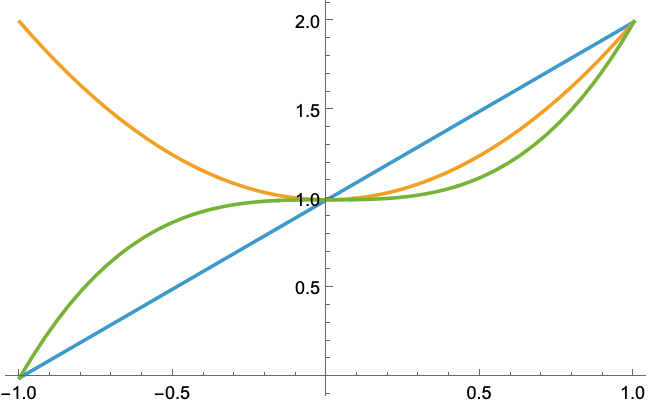
Tablefor PlottingTf = Table[x^n + 1, {n, 3}]Plot[Tf, {x, -1, 1}]
ListColors = Table[RandomColor[], {i, 5}]TG = Table[Plot[ft[t], {t, 0, 2 Pi}, PlotStyle -> C], {C, ListColors}]
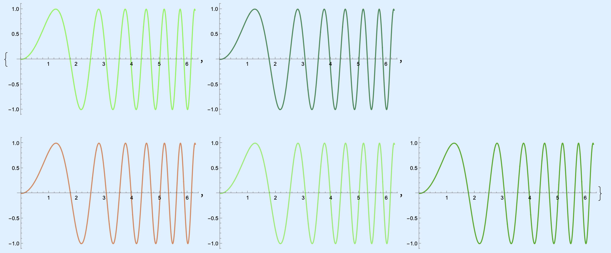
- เอาไปแสดงผลบางอันได้เช่น
{TG[[2]], TG[[5]]}GraphicsRow[{TG[[2]], TG[[5]]}](เหมือนข้างบนเป๊ะ)
- เอาไปแสดงผลบางอันได้เช่น
Define a Variable
x1 := 2จะไม่โชว์ value แต่แค่ define variable, ถ้าอยากให้ display ใช้ = เฉย ๆ นะx2 = 2อันนี้เวลา Run cell มันจะโชว์ Value ออกมาด้วยx2 = 2;ใส่ Semicolon เป็นการ Suppress output ไม่ให้ออกมาClear[x1]เป็นการ Clear Variable— จะได้เอา Variable นี้ไปใช้ต่อได้ในอนาคต555- ถ้าสมมติมี Function ที่ติดตัวแปลใช้
Simplifyให้มันดูง่ายขึ้นได้ → ก็จะถ้ามีวงเล็บมันก็จะกระจายเข้าไปทั้งหมด
Define a Function
1 Variable (2D)
f[x_] := x^2(สังเกตว่า มี Underscore ด้วยนะ) หรือจะf[x_] = x^2เฉย ๆ ก็ได้เหมือนกัน แค่จะมี Output ออกมาให้ดูด้วยนั่นเอง
2 Variables+ (3D)
- Function of two or more variables
f[x_, y_] := x^2 + y^2f2DL[{x_, y_}] := x^2 + y^2(สามารถ provide argument เป็น List ได้ เผื่อมีตัวแปรเยอะ ๆ)f2DL[ArgL]Call function with one argument ได้เลย โดยมีค่าเป็น List อยู่ข้างใน ก็จะ evaluate ค่าออกมาให้ โดยArgL = {2, 5}
fL[a_] := a[[1]]^2 + a[[2]]^2แล้วเวลาเรียกดูค่าหรือว่าอะไรก็ให้ listfL[{1, 3}]แบบนี้- แต่ถ้าเรา provide exceeding argument
fL[{1, 3, 5}]มันจะ ignore5ไปเลย
- แต่ถ้าเรา provide exceeding argument
Pure Function
- สามารถ Define Function แบบนี้ได้เหมือนกัน
(3 + #) &[x]โดย Output ออกมาเป็น3+xf3 = 3 + # &อย่าลืม end of the body ก็คือ & ด้วยfs = #1 + #2 + #3 &fs[1, 2, 3]Worksfs[1, 2, 3, 4]Also works (4 will be ignored)
- ==Pure Function ห้าม Define แบบมี Variable อยู่แล้วนะ
f[x_] = Sin[#] &ไม่ได้้้==
Plotting
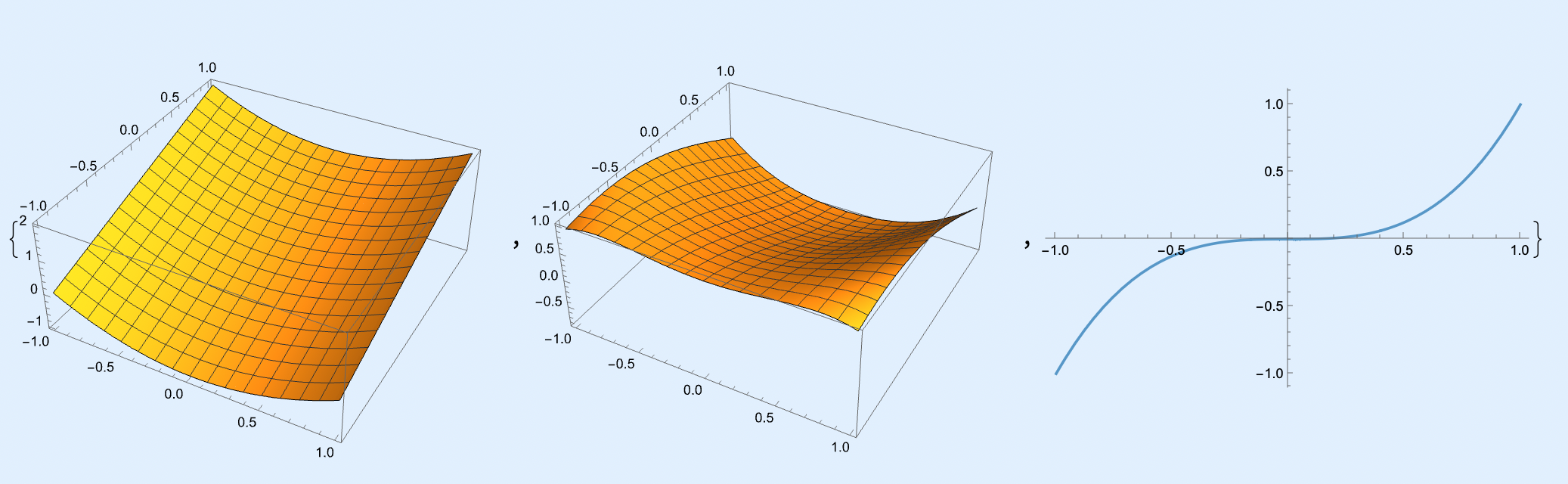
- เมื่อใช้ Plot อะไรแล้วมันจะออกมาเป็น Graphics ใช่มั้ย แล้วสามารถเอามาโชว์เป็น List ได้เลย
- เช่น
PL = {PL1, PL2, Plot[x^3, {x, -1, 1}]}
- เช่น
Function
Showเอาไว้ใช้ Show Graphics ไม่ว่าจะเป็นอันเดียวหรือว่าหลาย ๆ อัน
- แต่เหมือนว่าต้องเป็น 2D, 3D อย่างใดอย่างหนึ่งเท่านั้นนน!
โดยสามารถPlotRange -> {{0, 4}, {-4, 2}}ได้ด้วย อย่างเจ๋ง
Plot Styles
Basic Plotting
2D Plots
- 1 Function
Plot[f[x], {x, -1, 1}]
- More Functions
Plot[{f1[x], f2[x]}, {x, -10, 15}, PlotStyle -> {Red, Blue}]
3D Plots
Plot3D[f[x, y], {x, -1, 1}, {y, -1, 1}]
Parametric Plots
L[t_] := {3 + t, 3 + 2 t}→ หรือดูเป็นMatrixForm[L[t]]ก็ได้
2D Parametric Plots
ParametricPlot[L[t], {t, -5, 5}]ParametricPlot[{Cir[t], Spi1[t]}, {t, 0, 4 Pi}, PlotStyle -> {Red, Blue}]- ถ้าอยาก Plot หลายอันให้โชว์ก็ทำแบบนี้
- Remark:
Cir[t],Spi1[t]อยู่ในรูปสมการ Parametric นะCir[t_] := {R*Cos[t], R*Sin[t]}
3D Parametric Plots
GSp = ParametricPlot3D[S1[u, v], {u, 0, 4}, {v, 0, 4}, PlotStyle -> Blue, MeshStyle -> White]- Where
S1[u_, v_] := {x1[u, v], y1[u, v], z1[u, v]}
- Where
Spiral (JUM)
x[t_] := R Cos[t]y[t_] := R Sin[t]z[t_] := tSpiral[t_] := {x[t], y[t], z[t]}ParametricPlot3D[Spiral[t], {t, 0, 50}, BoxRatios -> 1, PlotStyle -> {Red, Thickness[0.001]}]
Polar Plots
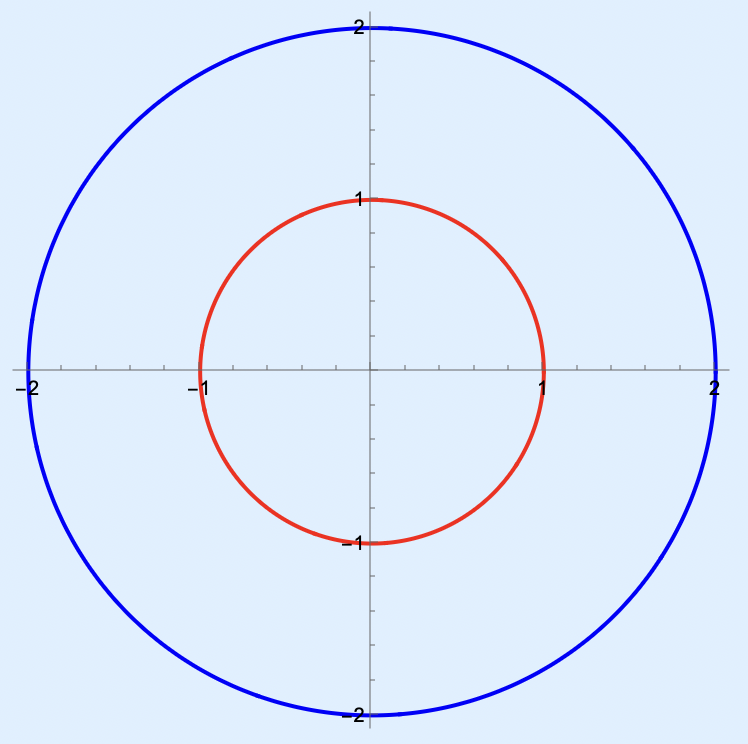
PolarPlot[R, {t, 0, 2 Pi}]โดยR = 1PolarPlot[2*Cos[2*t], {t, 0, 2 Pi}]PolarPlot[{R1, R2}, {t, 0, 2 Pi}, PlotStyle -> {Red, Blue}]โดยR1 = 1และR2 = 2– Several curve in PolarPlot
Spherical Plots
SphericalPlot3D[{fR1, fR2, fR3}, {t, 0, Pi}, {p, 0, 3 Pi/2}]
Revolution Plots
RevolutionPlot3D[{x[t], y[t]}, {t, 0, 2 Pi}, BoxRatios -> 1]- Revolve a function curve around the axis
- นึกให้เห็นภาพคือถ้า y = x, ก็จะออกมาเป็นกรวย
Density and Contour Plots
Density Plot
- A Density Plot shows the height of the surface in the z direction by the color intensity
Gdensity1 = DensityPlot[fe[x, y], {x, -2, 2}, {y, -2, 2}]
Showคนละ Type ของ GraphShow[GraphicsRow[{Gdensity1, Gsurplot1}]]
Contour Plot
Gcontour1 = ContourPlot[fe[x, y], {x, -2, 2}, {y, -2, 2}]Show[GraphicsRow[{Gdensity1, Gsurplot1, Gcontour1}]]Gcontour14 = ContourPlot[fe[x, y], {x, -2, 2}, {y, -2, 2}, Contours -> {1, 0.5, 0.4, 0.7}, ContourLabels -> True, ContourShading -> False]- จะได้เป็นขาวดำ, CoutourShading อะ
SliceContourPlot3D + SliceDensityPlot3D
Gslice1 = SliceContourPlot3D[fe[x, y], z == 0, {x, -2, 2}, {y, -2, 2}, {z, -2, 2}]→ อันนี้จะทำให้มาอยู่ใน 3D แล้วสุดท้ายก็สามารถShowกับกราฟของจริงได้Show[{Gslice1, Gsurplot1}, PlotRange -> {Automatic, Automatic, {0, 3}}]
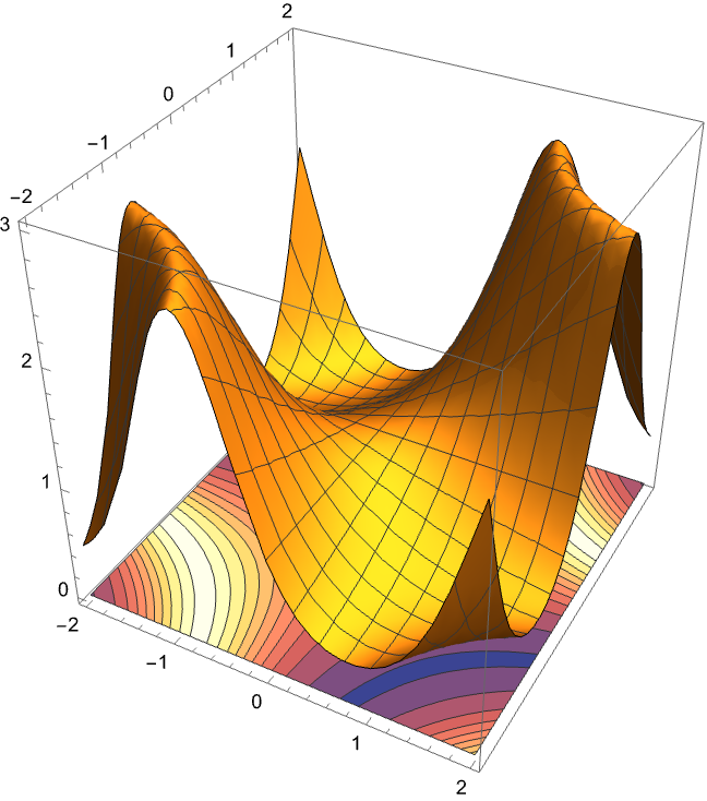
RegionPlot + RegionPlot3D
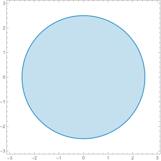
RegionPlot[x^2 + y^2 < R, {x, -3, 3}, {y, -3, 3}]- ถ้าเป็น
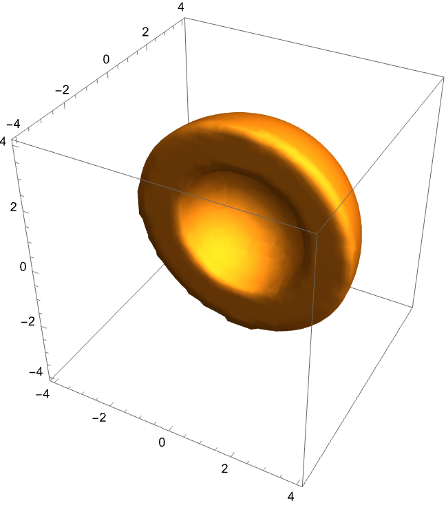
RegionPlot3Dมันก็จะมีเนื้อข้างในด้วย
ListPlot
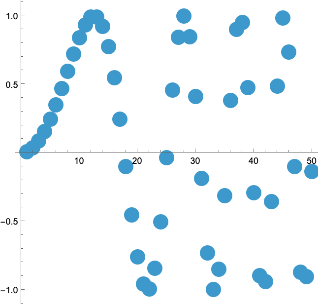
- ก็คือเอาค่าที่อยู่ใน List มา Plot เป็นจุด ๆ
- อาจจะเอาข้อมูล Import มา
ListPlot[Largedata, PlotStyle -> PointSize[0.05], AspectRatio -> 1]
Interpolation
data1 := {1, 2, 5, 7, 8, -5, 6, -3}- ถ้ากำหนด Data แบบนี้ แต่ละตัวจะเป็นของ x = 1, 2, 3, … ไปเรื่อย ๆ — ค่า y ก็จะเป็นในตาม
data
plot1points = ListPlot[data1, PlotStyle -> {PointSize[0.05], Red}] f1 = Interpolation[data1, Method -> "Spline"]; Table[f1[i], {i, Length[data1]}] plotf1 = Plot[f1[x], {x, 1, Length[data1]}]- ถ้ากำหนด Data แบบนี้ แต่ละตัวจะเป็นของ x = 1, 2, 3, … ไปเรื่อย ๆ — ค่า y ก็จะเป็นในตาม
- data2 =
{{1, 1}, {2, 3}, {-1, -3}, {7, 0}, {4, -4}};เรากำหนดแบบนี้ก็ได้ ระบุเป็น x, y coordinate ไปเลย!- ถ้าให้มาเป็น Coordinate แบบนี้ก็มีอยู่สองวิธีนะที่จะทำได้
- ทำคล้าย ๆ กับข้างบนเลย ก็คือจับทั้ง Data ยัดเข้า Interpolation เลย
interpFunc = Interpolation[data2, Method -> "Spline"]; plotf1 = Plot[interpFunc[x], {x, 1, 7}]- ต้องแยกแกนออกมาเป็น x, y ก่อน แล้วค่อยเอาใส่ Interpolation จ้า
xd0 = Transpose[data2][[1]];
yd0 = Transpose[data2][[2]];

sd0x = Interpolation[xd0, Method -> "Spline"];
sd0y = Interpolation[yd0, Method -> "Spline"];

Traj0[t_] := {sd0x[t], sd0y[t]}
plot0t = ParametricPlot3D[Traj0[t], {t, 1, 8}];
- ถ้าให้มาเป็น Coordinate แบบนี้ก็มีอยู่สองวิธีนะที่จะทำได้
ถ้าเป็น 3D ต้องทำแบบที่ 2 เท่านั้น!!!! แบบแรกทำไม่ได้นะ เข้าใจมั้ย?
Approximation & Fitting
- สมมติว่าเรามี Point ไปเรื่อยเลย เป็นข้อมูลหลาย ๆ อย่างอยู่ในรูป
data = {{0, 1}, {1, 0}, {3, 2}, {5, 4}};- เราสามารถเรียก
lm = LinearModelFit[data, x, x]→ หาสมการจากหลาย ๆ จุด คล้าย ๆ Linear Regression - Output ของ
lmจะออกมาเป็นคล้าย ๆ Model →FittedModel[0.186441 + 0.694915x] - จะ Obtain the functional form ให้ใช้
Normal[lm]หรือว่าlm[t]ไปเลย (แบบที่อาจารย์ใช้) ก้จะได้สมการ Linear Regression ใน Form ของ t ออกมา
- เราสามารถเรียก
- แต่ถ้าอยากให้มัน Fit กับจุดเรามาก ๆ มาดูใหม่ที่
lm = LinearModelFit[data, x, x]- เราสามารถเพิ่ม Degree ของสมการที่เราอยากให้มันออกมาได้ เช่น
lm = LinearModelFit[data, {x,x^2,x^3}, x]สมการก็จะออกมามี Degree ตามที่เราอยากได้แล้ว - จริง ๆ ไม่จำเป็นต้องอยู่ในรูป
x, x^2, x^3ไรงี้ก็ได้นะ อาจจะอยู่ในรูป ยังได้เลย 555
- เราสามารถเพิ่ม Degree ของสมการที่เราอยากให้มันออกมาได้ เช่น
WTF is FitResiduals?
- FitResiduals gives the difference between the response values in the input data and the fitted values
Graphics and Visualization
Colors and Styling
RandomColor[]- returns a random RGB colorRGBColor[{10/255, 132/255, 255/255}]- returns custom RGB color
Points
Define Point(s)
Pn1 = Point[{1, 2}, VertexColors -> Red]Pn2 = {{1, 2}, {3, 4}, {2, -1}}
Show Point
Graphics[{PointSize[0.15], Point[{1, 2}]}, PlotRange -> 3, Axes -> True]Graphics[{PointSize[0.05], Pn1}, Axes -> True]Graphics[{Red, PointSize[0.1], Point[Pn2]}, Axes -> True, AspectRatio -> 1]Graphics[{PointSize[0.1], Point[Pn2, VertexColors -> Col]}, Axes -> True, AspectRatio -> 1]- โดย
Colจะเป็นCol = {Red, Blue, Orange}
- โดย
Graphics3D
Points12 = Point[{p1, p2, p3}, VertexColors -> Colors12]- Output:
Point[{{1, 1, 1}, {1, 2, 2}, {2, 3, 3}}, VertexColors -> {Red, Green, Blue}]
- Output:
Graphics3D[{PointSize[0.05], Points12}, PlotRange -> 3.2, Axes -> True]
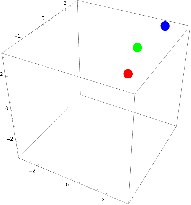
P10 = Table[fRandom3D[], {i, 10}]ใช้ Table, เอาจุดเข้าเป็น Array จาก FunctionfRandom3D[]fRandom3D[] := {0.5 - Random[], 0.5 - Random[], 0.5 - Random[]}
Points10 = Point[P10],Lines10 = Line[P10]GP10 = Graphics3D[{{Red, PointSize -> 0.05, Points10}, Lines10}, Axes -> True]
Text
GP50ST = Graphics3D[Text["My spiral", P50S[[50]]], BoxRatios -> 1]- หรือถ้าอยากใส่ Font
T1 = Style["My Spiral\nStaircase", Large, Bold, Blue, FontFamily -> "SF Mono"]GP50ST1 = Graphics3D[Text[T1, P50S[[Npoints]]], BoxRatios -> 1]
Sphere
Sphere[p]represents a unit sphere centered at the point p.Sphere[p, r]represents a sphere of radius r centered at the point p.Sphere[{p1,p2,...}, r]represents a collection of spheres of radius r.
Cylinder
- ต้อง Provide 2 coordinate point and a radius
Graphics3D[Cylinder[{{1, 1, 2}, {1, 1, 3}}, 2], Axes -> True, AxesOrigin -> {0, 0, 0}, Boxed -> False]
Arrow
A1 = Arrow[{{1, 0}, {2, 1}, {3, 0}, {4, 1}}]Graphics[{Blue, A1}, Axes -> True]- Connects the points into a sequence of arrows/lines
GLines = Graphics[Line[P10], ImageSize -> Small, Axes -> True]
Platonic Solids
Graphics3D[{Red, Tetrahedron[]}]Graphics3D[{Yellow, Octahedron[]}]Graphics3D[{Green, Icosahedron[]}]Graphics3D[{Blue, Icosahedron[]}]Graphics3D[{Brown, Dodecahedron[]}]

- โดยสุดท้ายก็สามารถไปทำให้มัน Move Along the curve ได้เหมือนกัน
MoveOctahedron[P_] := Graphics3D[{Yellow, Opacity[0.8], Octahedron[P, 2]}]- โดยสุดท้ายก็สามารถแทน
Pด้วย{sx4[t], sy4[t], sz4[t]}ประมาณนี้!
RegularPolygon
PTri = {Red, RegularPolygon[{0, 0}, 1, 3]}{0, 0}คือ Origin1คือ Size3คือจำนวนด้าน
- ก็สามารถเอามาประยุกต์ใช้กับ Geometric Transformation ได้
T[a_] := Graphics[{GeometricTransformation[PTri, RotationTransform[a]]}, Axes -> True, PlotRange -> 3]Manipulate[T[t], {t, 0, 2*Pi, 0.1}]- แต่คือถ้าตรงนี้ Origin อยู่ข้างนอก มันก็จะหมุนรอบทั้งหมดเลยนะ ไม่ใช่แค่หมุนรอบตัวเอง
Data Handling
Arrays
-
Array[f, 10, {1, 10}]— generates a list using n values from a to b -
f[x_] := {x, Sin[x^2]}P10 = Array[f, 10, {0, 1.}]{{0., 0.}, {0.111111, 0.0123454}, {0.222222, 0.0493626}, ...
Mapping Functions
Map[Sin, {0, Pi/4, 3 Pi/2}]— ก็เหมือน for loop เอาแต่ละตัวเข้าไปแทน (แต่ไม่ได้ Iterate over a range)- สามารถไป Mix & Match กับอะไรก็ได้เช่นพวกสี + ตำแหน่งงี้
Importing Data
Largedata := Import["experiment.txt", "List"]อันนี้ก็เหมือน import มา as a listSetDirectory["filepath”]
- สามารถเอามา Plot ใช้ ListPlot
Animations
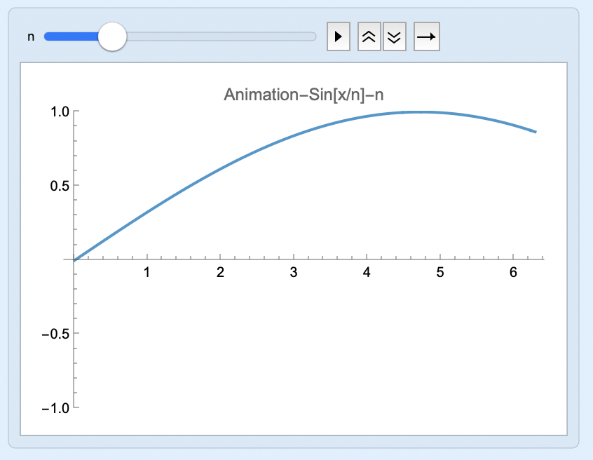
Animate[YourPlot[animationParameter], {animationParameter, pmin, pmax, step}], AnimationRunning -> False
fn[x_, n_] := Sin[x/n]Animate[Plot[fn[x, n], {x, 0, 2 Pi}, PlotPoints -> 100, PlotRange -> 1, PlotLabel -> "Animation-Sin[x/n]-n"], {n, 1, 10, 1}, AnimationRunning -> False]
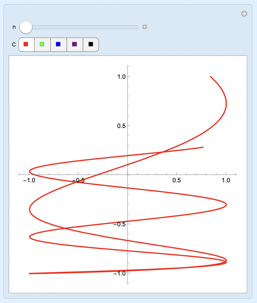
Manipulate[ParametricPlot[S1[t, n], {t, 0, 5}, PlotStyle -> C], {n, 1, 5, 0.1}, {C, Color1}]- โดยที่
Color1 = {Red , Green, Blue, Purple, Black}
- โดยที่
ToExpression
- แต่ถ้าเรา Define แบบนี้
ColorT = {"Red" , "Green", "Blue", "Purple", "Black"}- สังเกตว่า เป็น Array of String
Manipulate[ParametricPlot[S1[t, n], {t, 0, 5}, PlotStyle -> ToExpression[C]], {n, 1, 5, 0.1}, {C, ColorT}]- ทำหน้าที่เปลี่ยนจาก “String” ให้เป็น Expression ธรรมดา
Dynamic
- The one that is automatically updated to always reflect its current value. This new kind of output is provided by the function
Dynamic Dynamic[x]- ถ้ามีบรรทัดด้านบน
x = 62หรือเราเปลี่ยนไปเรื่อย ๆ มันก็จะเปลี่ยนให้เองเลย เหมือนมัน watch for changes อยู่แล้ว
- ถ้ามีบรรทัดด้านบน
Slider
-
{Slider[Dynamic[s], {-4, 75, 3}] , Dynamic[s]}- var ใน slider ต้องเป็น dynamic

- var ใน slider ต้องเป็น dynamic
-
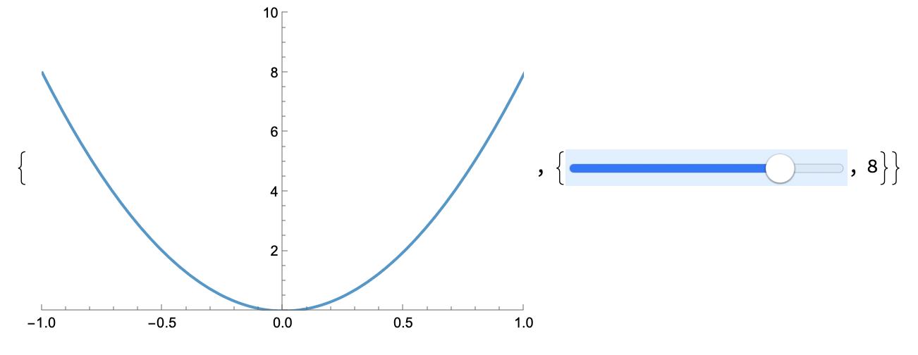
{Dynamic[Plot[f[x, a], {x, -1, 1}, PlotRange -> {{-1, 1}, {0, 10}}]], {Slider[Dynamic[a], {0, 10, 1}, Background -> LightBlue], Dynamic[a]}}- โดย
f[x_, a_] := a*x^2
- โดย
-
หรือจะแยกฟังก์ชันแต่ละตัว แล้วก็เอามารวมกัน
Sm6 := {Slider[Dynamic[m6], {0, 10, 1}, Background -> LightBlue], Dynamic[m6]}Sn6 := {Slider[Dynamic[n6], {0, 10, 1}, Background -> Green], Dynamic[n6]}{Dynamic[P6[n6, m6]], Sm6, Sn6}
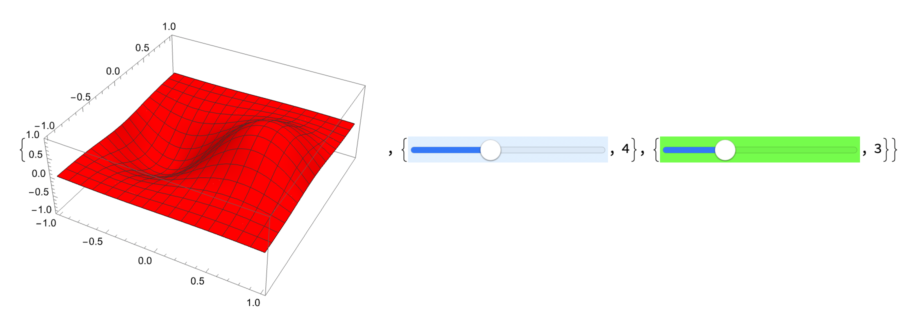
-
VerticalSliderก็มีนะ! เหมือนกันเลย แค่เป็นแนวตั้ง
Toggler
- ก็เหมือน Toggle เป็นปุ่มเดียว จะโชว์ Text ต่าง ๆ ปรับแล้วก็เพิ่มไปทีละ 1 เรื่อย ๆ
TL7 = Table[0.5*i, {i, 10}]Toggler[Dynamic[a], TL7, Background -> Blue, BaseStyle -> White]
RadioButtonBar
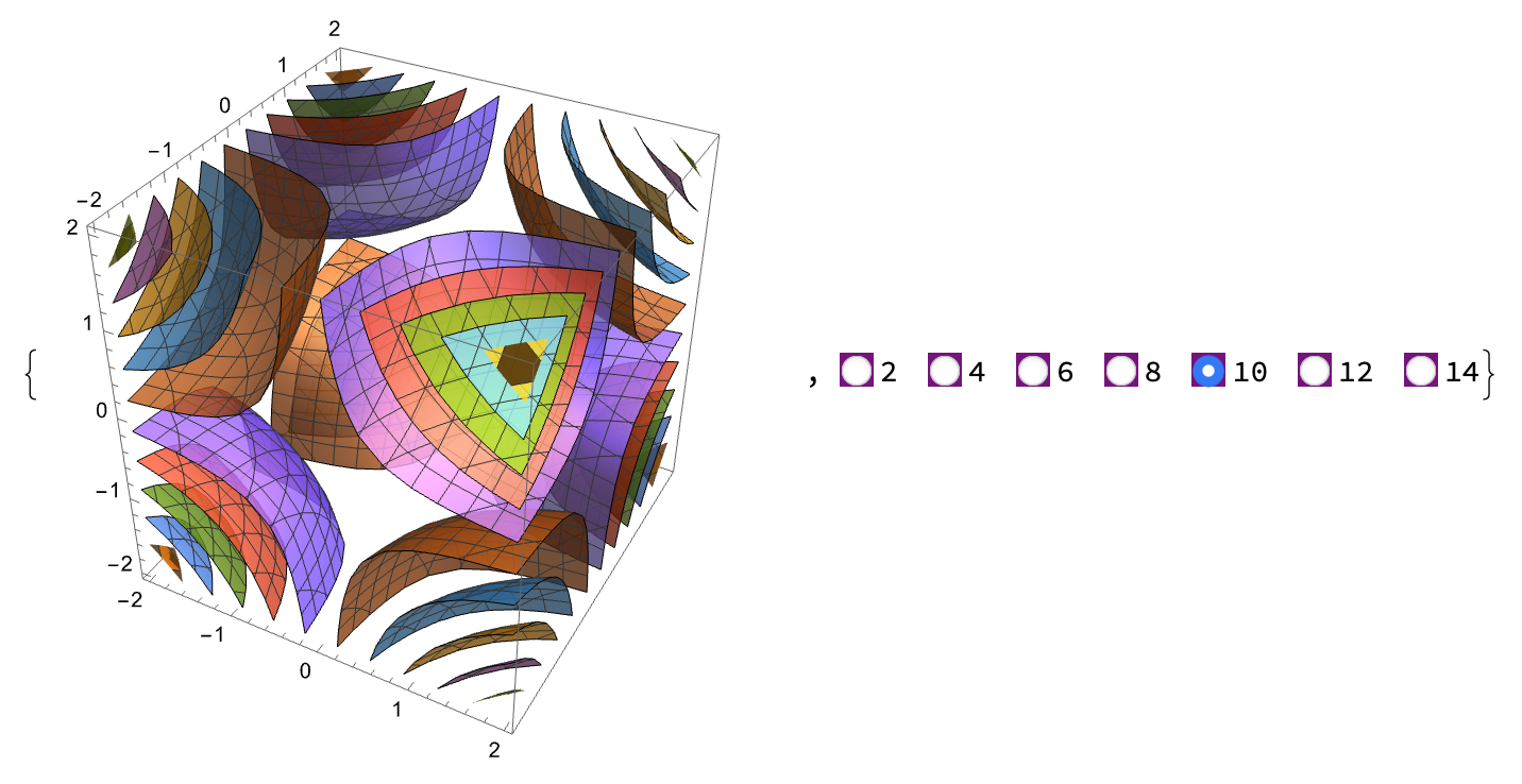
RBar7 := RadioButtonBar[Dynamic[c1], T7n, Background -> Purple]{Dynamic[plot7n[c1]], RBar7}
PopupMenu
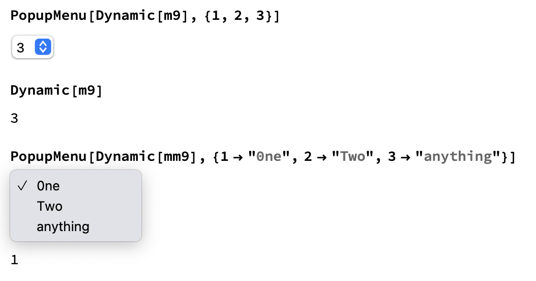
- ลักษณะจะเป็น Drop Down Menu ลงมา
SetterBar
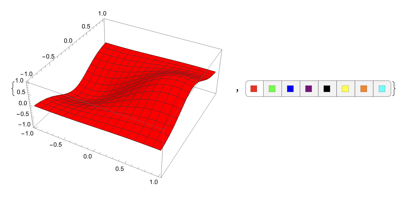
SB11 := SetterBar[Dynamic[color11], {Red, Green, Blue, Purple, Black, Yellow, Orange, Cyan}]{Dynamic[plot101[color11]], SB11}
ColorSlider
CS12 = ColorSlider[Dynamic[color12]]
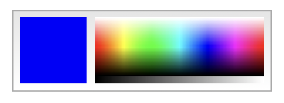
Control
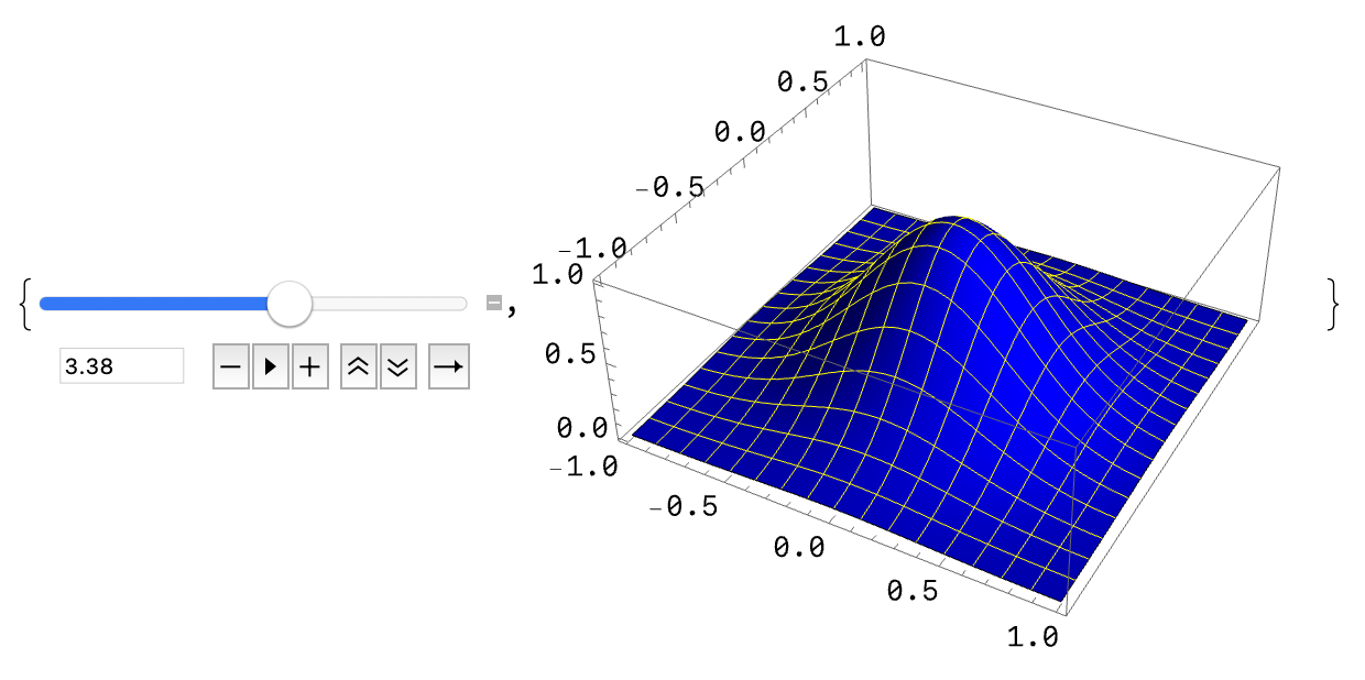
- Step is automatic
- เหมือนกับ Slider แต่ไม่ต้อง Provide Step ให้
C5 := Control[{a5, 1, 5}]{C5, Dynamic[plotf[Blue, a5]]}
Slider2D
#FinalExam
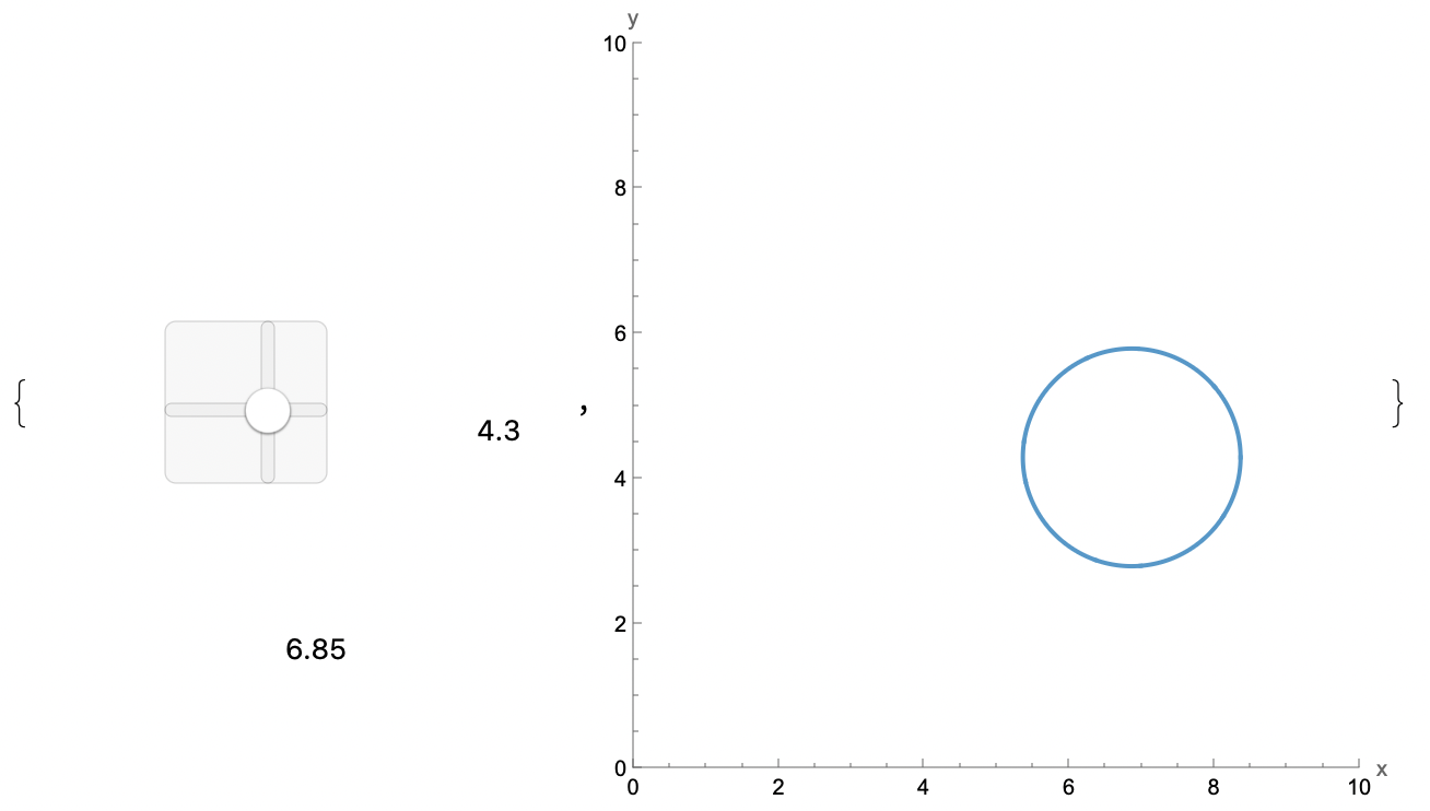
{Slider2D[Dynamic[z], {{0, 0}, {10, 10}}, ImageSize -> Large, Appearance -> "Labeled"], Dynamic[PlotC[z[[1]], z[[2]]]]}
- เวลาเรียกใช้ก็เหมือน Access ค่าจาก Array ได้เลย
Plot a Plane
- อยาก Plot
z = 3→Plot3D[3, {x, -1, 1}, {y, -1, 1}]
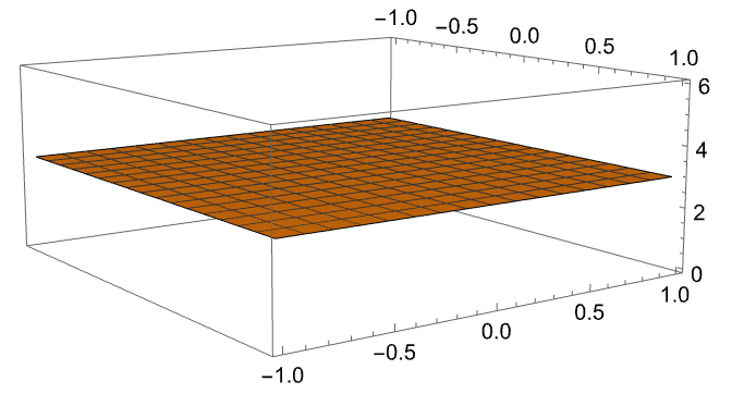
- แต่ถ้าอยาก Plot Plane บนแกน
xหรือyต้องใช้ParametricPlot3Dx = 5S[u_, v_] := {5, u, v}Z1 = ParametricPlot3D[S[u, v], {u, -1, 1}, {v, -1, 1}, BoxRatios -> 1]
y = 5S[u_, v_] := {u, 5, v}ParametricPlot3D[S[u, v], {u, -1, 1}, {v, -1, 1}, BoxRatios -> 1]
zก็ทำได้เหมือนกัน แต่Plot3Dเหมือนเป็น Shortcut (ลักไก่)
Module
f[Input_] := Module[{x, y, ...}, expr1; expr2; Output]- เข้าใจละ ๆ มันก็เหมือนกับเป็น Compound function (เราสามารถเขียน Function หลาย ๆ ตัวให้มันทำงานเรียงลำดับกันได้) → แล้วก็ให้ Output เรามา
- โดย
{x, y, ...}เป็นเหมือน Variable ของ Function ทั้งหมด- โดยทุกตัวจะถูก Treat เป็น Local variable ของ Module นี้!!
Example
f0[a_, b_] := Module[{s}, s = a + b; s += 1; s]
โดยอันนี้มี Local Variable เป็น s ตัวเดียว— จะโดนเอาไป a + b ก่อน แล้วบวก 1 อีกที ทำตามลำดับ— ส่วน s ท้ายสุดคือ Output variable ของเรา มันก็จะโชว์ค่าสุดท้ายของ s นั่นเองง!!
fib[n_] := Module[{f},
					f[1] = f[2] = 1;
					f[i_] := f[i] = f[i - 1] + f[i - 2];
					f[n]
				]
หรืออันนี้โหดหน่อย ก้เอาไปใช้กับ Fibonacci 5555555
f1[N_] := Module[{T}, T = Table [i, {i, N}]; T]
จะเอาไปประยุกต์ใช้กับ Function อื่น ๆ ก็ยังได้เช่น Table เวลาเราอยากได้ออกมาก็แค่พิมพ์ f1[5] จะได้ออกมาเป็น {1, 2, 3, 4, 5}
f2[N_] := Module[{T, S}, T = Table [i, {i, N}]; S = Sum[T[[i]], {i, N}]; {T, S}]
มาดูที่เป็นหลาย Local variables กันบ้าง, เวลา Output จะได้ออกมารูปแบบนี้ {{1, 2, 3, 4, 5}, 15}
→ อีกอันให้ Table อีกอันให้ Sum
สุดท้ายก็อาจจะเอาไปทำอะไรก็ได้ / อาจจะเกี่ยวกับ Interpolation ที่ต้องเขียนเยอะ ๆ ก็เอามาลดได้เป็น Function เดียว เรียกได้หลาย ๆ รอบเลย 555 สุดยอดดดดด
Condition Statement
If
- The "If" statement is given by
If[condition, TRUE (t),FALSE (f)]gives t if condition evaluates to True and f if it evaluates to False.
Example
div1[x_, y_] := If[y == 0, "∞", x/y ]→"∞"เป็นแค่ String นะ (เอาไว้เช็ค กันไว้)div1[1, 4]=div1[2, 0]=
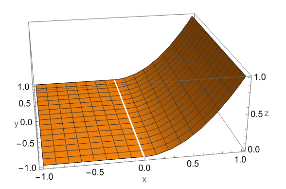
- จะเอามา Plot Surface แบ่งกันก็ได้ ครึ่งนึงสมการนี้ อีกครึ่งอีกสมการ
S51[u_, v_] := u^2S52[u_, v_] := 0S5[u_, v_] := If[u > 0, S51[u, v], S52[u, v]]Plot3D[S5[u, v], {u, -1, 1}, {v, -1, 1}]- แต่มันจะมีเส้นแบ่งสีขาว ๆ ตรงกลาง ดังนั้นต้องเพิ่ม
Plot3D[S5[u, v], {u, -1, 1}, {v, -1, 1}, Exclusions -> None]
- แต่มันจะมีเส้นแบ่งสีขาว ๆ ตรงกลาง ดังนั้นต้องเพิ่ม
- สามารถเอาไปประยุกต์ให้มันเปลี่ยนสีไปเรื่อย ๆ ก็ได้นะ!
Testing Expressions
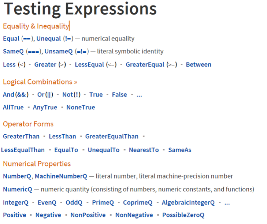
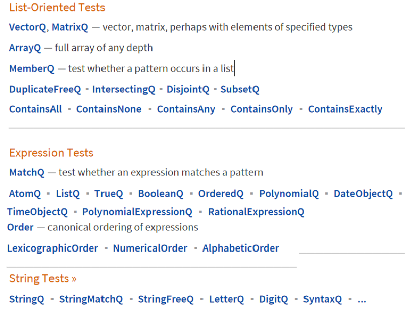
check1[x_] := If[IntegerQ[x] && NumberQ[x] && Positive[x], 1/(1 + x), "error"]
Looping
For[i = 0, i < 4, i++, Print[i]]For[init, test, incr, body]- ถ้าสมมติ
bodyซับซ้อนเช่นต้องIfซ้อน ก็ทำเหมือนมันเป็น Closure 5555 For[i = 2, i <= N1 - 1, i++, {If[Mod[N1, i] == 0, {Print[i], Break[]}]}]
- ถ้าสมมติ
Geometric Transformations
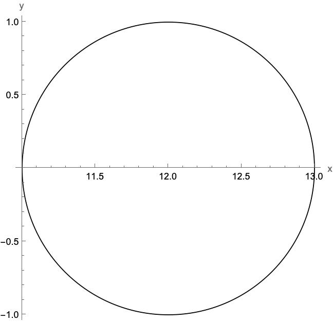
Translations
Graphics[{GeometricTransformation[Circle[], TranslationTransform[{12, 0}]]}, Axes -> True]
Superposition of the Transformations
ต้องมี Keyword คำว่า
Composition
- รวมกับทั้ง Translation, Rotation — หรือจะแค่รวมกันหลาย ๆ อัน ในอันเดียวก็ได้!
Graphics[{GeometricTransformation[Circle[], Composition[TranslationTransform[{12, 0}], TranslationTransform[{0, 12}]]]}, Axes -> True]- Multiple transforms applied to 1 object
Graphics[{GeometricTransformation[Circle[{0, 0}, 3], {TranslationTransform[{6, 0}], TranslationTransform[{12, 0}]}]}, Axes -> True]
Notes
จากที่สังเกตคือเหมือนใน Composition ถ้าเราจะจินตนาการ คือเหมือนมันจะทำ จาก หลัง → หน้า
จริงหรือ (เสียงภาณุวงค์) จริงงงงง! Confirmed!
Example
Translation along the curve (parametric)
- สมมติว่ามี Curve:
Curve6[t_] := {2 Cos[3 t], 2 Sin[2 t]} - สามารถให้ Object มันวิ่งตาม Curve ได้แบบนี้
TriCurve6[a_, t_] := GeometricTransformation[ObjectTri, Composition[TranslationTransform[Curve6[t]], RotationTransform[a]]]- แล้วอย่างที่บอกว่ามันอ่านจาก หลัง → หน้า ดังนั้นอันนี้มันจะ หมุนรอบตัวเองก่อน แล้วก็ Translation ไปรอบ ๆ Curve
- แล้วถ้าจะให้โชว์ Curve + Object ด้วยก็:
ShowAll6[a_, t_] := Show[FTri6[a, t], PC6] Manipulate[ShowAll6[10*t, t], {t, 0, 2 Pi - 0.0001, 0.1}]
Matrix Algebra + Geometric Transformations
Example
Example 1: Rotate a Point Around a Specific Point Using Matrix Algebra
RR1 = {0, 3.5};

Paround1 = {-5, -5};

PointH1 = {0, 0, 1}; (* The 1 is used to enable affine transformations (like translation) with matrices. จำไปเลยว่า 2D ต้องเติม 1 ให้เป็น 3D *)

RP1 = Composition[TranslationTransform[Paround1], RotationTransform[a], TranslationTransform[RR1]] (* โดยอันนี้เข้าใจง่ายมาก เดี๋ยวอธิบายด้วยภาพ ยืดตามหลักจาก หลัง -> หน้า อย่างที่บอกนะ *)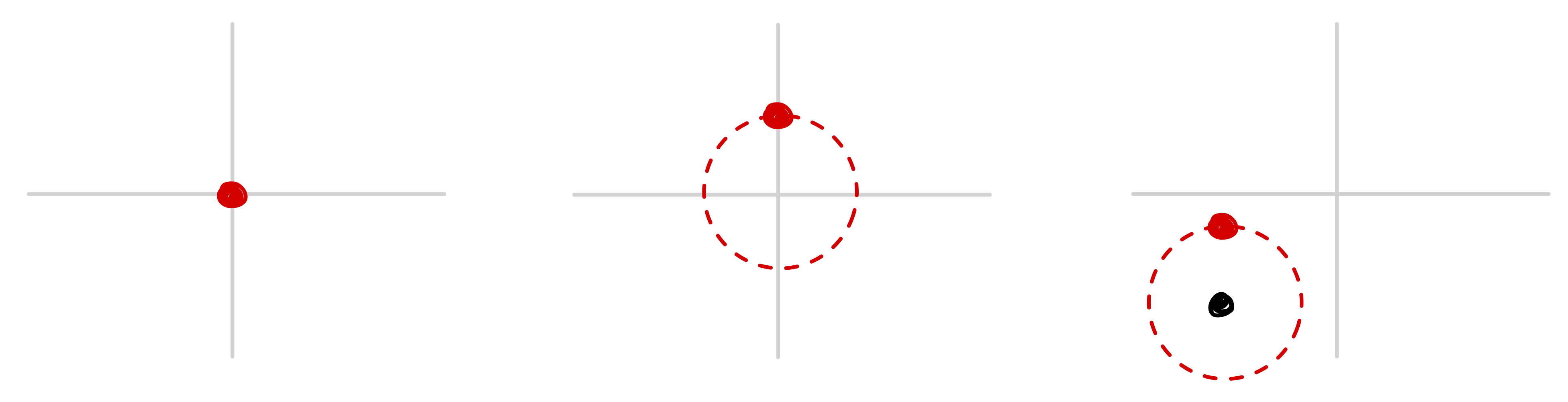
MP1 = TransformationMatrix[RP1] (* Converts that composite transformation into a symbolic matrix representation *)

MFP1[a_] := Evaluate[MP1] (* Wraps that matrix into a function of angle a ทำให้เป็น Function *)

MatrixForm[MFP1[a]] (* ลอง Print ออกมาดู ตอนนี้เป็น Matrix แล้ว *)

PR1[t_] := (MFP1[t] . PointH1)[[1 ;; 2]] (* This gives the actual 2D coordinates after rotation *)

MatrixForm[PR1[t]] (* จะได้มาเป็น Column สุดท้าย (2D) *)

PParound1 := {PointSize[0.05], Red, Point[Paround1]}

AnimPR1[t_] := Graphics[{{PointSize[0.05], Point[PR1[t]]}, PParound1}, Axes -> True, PlotRange -> 15]

Manipulate[AnimPR1[t], {t, 0, 2*Pi}]
Example 1’: Geometric Transformation of a Point Around a Point Using Primitives
เหมือนเมื่อกี้ แต่ว่า Approach นี้ง่ายกว่า ไม่ได้ใช้ Matrix แต่อย่างใด ใช้ geometric transform
RR1 = {0, 3.5};
Paround1 = {-5, -5};
myPoint = {0, 0}; (* อันนี้ไม่ต้องเติม 1 มาแล้วนะ no H-coordinate *)

GT1[a_] :=
 GeometricTransformation[Point[myPoint],
  Composition[TranslationTransform[Paround1], RotationTransform[a],
   TranslationTransform[RR1]]]

PParound1 := {PointSize[0.05], Red, Point[Paround1]}

myAnim1[t_] :=
 Graphics[{{PointSize[0.05], GT1[t]}, PParound1}, Axes -> True,
  PlotRange -> 15]

Manipulate[myAnim1[t], {t, 0, 2 Pi}]
Example 1’′: Alternative Rotation Using RotationTransform[a, p]
ก็เหมือนกัน เป็นข้อเดียวกัน แต่ Alternative approach ให้มันรอบจุดเอา
RR1 = {0, 3.5};
Paround1 = {-5, -5};

Pinit1 = {-5, -5} + {0, 3.5} (* Computes the actual initial point's position before rotation *)

Graphics[{PointSize[0.05], Point[Pinit1]}, Axes -> True, PlotRange -> 15] (* Visualizes the original point's location. *)

GT2p[a_] :=
 GeometricTransformation[Point[Pinit1], RotationTransform[a, Paround1]] (* Applies a simpler transformation: rotate Pinit1 around Paround1 using built-in function. *)

myAnim2p[t_] :=
 Graphics[{PointSize[0.05], GT2p[t], PParound1}, Axes -> True,
  PlotRange -> 15]

Manipulate[myAnim2p[t], {t, 0, 2 Pi}]
Example 2: Rotate a Curve Using Matrix Algebra
f2[x_] := x^2 (* Defines the original function *)

Plot[f2[t], {t, -1, 1}] (* Plot[f2[t], {t, -1, 1}] *)

RT2 = RotationTransform[a] (* Creates a symbolic 2D rotation around the origin. *)

M2 = TransformationMatrix[RT2]
M2F[a_] := Evaluate[M2]

S2H[t_] := {t, f2[t], 1}
S2H[s]

PR2[a_, t_] := (M2F[a] . S2H[t])[[1 ;; 2]] (* ทำให้เหลือ 2 มิติ ต้องทำตลอด *)
MatrixForm[PR2[a, t]]

p2[a_] := ParametricPlot[PR2[a, t], {t, -1, 1}, PlotRange -> 1]

Zero = {Red, PointSize[0.05], Point[{0, 0}]}
Zero2 = Graphics[Zero];

p2All[t_] := Show[p2[t], Zero2]
Manipulate[p2All[a], {a, 0, 2 Pi}]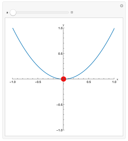
Example 3: Dual Rotation of a Parametric Curve
(* Define the pivot and radius vector *)
Paround5 = {5/2, 5/2};
RR5 = {0, 3/2};

(* Define the parametric curve *)
S5[t_] := 2 {Sin[2*t], Cos[3*t]}
S5G = ParametricPlot[S5[t], {t, 0, 2 Pi}, Axes -> False] (* Plot *)

S5P = S5G[[1]]; (* Convert the plot into primitives *)
Graphics[S5P] (* Quick check of the primitive *)

Object5 = {Zero, S5P}; (* Zero คือ {Red, PointSize[0.05], Point[{0, 0}]} *)
Graphics[Object5]

RT5[a_, b_] :=
  GeometricTransformation[Object5,
   Composition[RotationTransform[a, Paround5],
    TranslationTransform[RR5], RotationTransform[b]]]; (* This creates a double rotation: one on itself, one around the pivot. *)

GParound5 = {Purple, PointSize[0.05], Point[Paround5]};
ShowAll5[a_, b_] :=  Graphics[{RT5[a, b], GParound5}, PlotRange -> 7, Axes -> True]

Manipulate[ShowAll5[a, b], {a, 0, 2 Pi}, {b, 0, 2 Pi}]
Example Basic 2D and 3D Transformations
Example 1: Rotate a Torus in 3D
R1 = 1; R2 = 2;
Tor = {Purple, Opacity[0.5], Torus[{0, 0, 0}, {R1, R2}]};
Zero3 = {Red, PointSize[0.06], Point[{0, 0, 0}]}; (* Mark the origin with a red dot. *)

Yrot = 2*{0, 1, 0};
ArY = {Thick, Green, Arrow[{{0, 0, 0}, Yrot}]}
AllTor = {Tor, Zero3, ArY} (* Group the torus, red origin point, and green arrow together. *)
Graphics3D[AllTor, Axes -> True, Boxed -> True] (* Display *)

Rot1Tor[a_] := GeometricTransformation[AllTor, RotationTransform[a, Yrot]]
(* Defines a function that rotates the torus and other objects around the vector `Yrot` by angle `a`. *)

Manipulate[
 Graphics3D[Rot1Tor[a], PlotRange -> 2, Axes -> True], {a, 0, 12 Pi}]
Zrot = 3 {0, 0, 1};
An = {2, 2, 0};
(* Rotation axis vector along Z, scaled by 3, and anchored at {2, 2, 0} *)
ArZ = {Thick, Red, Arrow[{An, An + Zrot}]};
AllTorZ = {Tor, Zero3, ArZ};
AllTor2 = {Tor, Zero3};
Graphics3D[{AllTor2, ArZ}, Axes -> True, Boxed -> True]
Rot2Tor[a_] := GeometricTransformation[AllTor2, RotationTransform[a, Zrot, An]]
Manipulate[
Graphics3D[{Zero3, ArZ, Rot2Tor[a]},
PlotRange -> {{-3, 7}, {-3, 7}, {-2, 3}}, Axes -> True], {a, 0, 12 Pi}]- Exercise Additionally rotate the Torus around its center in the Y direction
Rot3Tor[a_] := GeometricTransformation[ AllTor2, Composition[ RotationTransform[a, Zrot, An], RotationTransform[6 a, Yrot] ] ]- Around
Zrotat anchorAnbya - Around
Yrot(at center) by6a(faster rotation)
Manipulate[ Graphics3D[{Zero3, ArZ, Rot3Tor[a]}, PlotRange -> {{-3, 7}, {-3, 7}, {-5, 5}}, Axes -> True], {a, 0, 2 Pi}] - Around
Example 2: Rotate a Surface Using a Rotation Matrix
We rotate the surface around the Z-axis using homogeneous coordinates and matrix algebra.
(* Define the surface function *)
f6[x_, y_] := x^2 - y^2

(* Lift to homogeneous coordinates (H-coordinates) *)
S6[u_, v_] := {u, v, f6[u, v], 1}

(* Rotation around Z-axis with symbolic angle 'a' *)
RTza6 = RotationTransform[a, {0, 0, 1}];

(* Extract the 4x4 transformation matrix *)
MCza6 = TransformationMatrix[RTza6];

(* Make a callable function of the matrix *)
FCza6[a_] := Evaluate[MCza6];

(* Apply the matrix to each point, then drop the homogeneous 4th component *)
RotS6[u_, v_, a_] := (FCza6[a] . S6[u, v])[[1 ;; 3]]

(* Optional: view a single transformed point as a matrix *)
MatrixForm[RotS6[u, v, a]]

(* Display red origin point for reference *)
GZero3 = Graphics3D[{Red, PointSize[0.1], Point[{0, 0, 0}]}];

(* Generate the rotated surface as a 3D plot *)
GRotS6[a_] := ParametricPlot3D[
  RotS6[u, v, a],
  {u, -1, 1}, {v, -1, 1},
  PlotRange -> 1.5
]

(* Animate the surface rotating around the Z-axis *)
Manipulate[
 Show[GRotS6[a], GZero3],
 {a, 0, 2 Pi}
]
Example 3: Fly a Cube Along a 3D Knot While Rotating
This example translates and rotates a cube along a complex 3D curve (a “knot”).
(* Define the 3D trajectory (a knot) *)
Ftra[t_] := {
  3/4 t (t^2 - 4) (t^2 - 11),
  t^4 - 12 t^2,
  1/30 t (t^2 - 1) (t^2 - 3) (t^2 - 9) (t^2 - 12)
}

(* Plot the trajectory curve *)
TrajCube = ParametricPlot3D[
  Ftra[t],
  {t, -3.5, 3.5},
  Axes -> False,
  Boxed -> False
]

(* Extract graphical primitives from the plot *)
TrajCubeP = TrajCube[[1]];

(* Combine a translation along the knot with a rotation about Z *)
RotTra[t_, a_] := Composition[
  TranslationTransform[Ftra[t]],
  RotationTransform[a, {0, 0, 1}]
]

(* Apply transformation to a large cube *)
CubeTrans[t_, a_] := GeometricTransformation[
  Cube[10],
  RotTra[t, a]
]

(* Show the cube and trajectory together *)
ShowFlyCube[t_, a_] := Graphics3D[
  {CubeTrans[t, a], TrajCubeP},
  PlotRange -> 40,
  Axes -> True
]

(* Animate the cube moving and rotating independently *)
Manipulate[
  ShowFlyCube[t, a],
  {t, -3.5, 3},
  {a, 0, 2 Pi}
]

(* Simplified version: rotate and move at the same rate *)
Manipulate[
  ShowFlyCube[t, t],
  {t, -3.5, 3}
]
Importing STL Models
What is it?
This example demonstrates how to:
- Import and visualize STL (stereolithography) files in Mathematica.
- Apply geometric transformations (like rotation and translation) to 3D models.
- Combine imported STL content with other 3D primitives using
Graphics3D.
Importing STL Files
Ex1 = Import["solid.stl", "PolygonObjects"];
Graphics3D[Ex1]

Spikey = Import["spikeymodel.stl", "PolygonObjects"];
Graphics3D[Spikey]"PolygonObjects"gives a structured geometric representation.- These are fully compatible with
Graphics3D.
Combining with Graphics3D Primitives
Sphere1 = {Yellow, Opacity[0.2], Sphere[{0, 0, 0}, 2]};
Zero = {Red, PointSize[0.08], Point[{0, 0, 0}]};

Comb1 = Graphics3D[{{Opacity[0.5], Spikey}, Sphere1, Zero}, Axes -> True]- Call
Import["filename.stl", "PolygonObjects"]to load an STL file. - Use
GeometricTransformationandRotationTransform/TranslationTransformfor moving the object. - Wrap everything in
Graphics3Dfor display.
สรุป Composition แบบรวบย่อ
- สมมติให้ คือ
TranslationTransform - สมมติให้ คือ
RotationTransform
GeometricTransformation[point, TranslationTransform[v]]- แค่เลื่อนแกนด้วย vector เท่านั้นเอง จะกำหนดเป็น {1,2} หรือ {-3,5} อะไรก็ว่าไป
GeometricTransformation[point, RotationTransform[θ]]- แบบนี้ก็แค่หมุนรอบตัวเอง รอบจุด Origin (0,0) ด้วยมุม
Composition[T, R]- หมุนก่อน แล้วค่อย เลื่อนไป
- เช่น: หมุน Object นึง (ซึ่งเราอาจต้องทำเป็น Primitive ก่อน แล้วเลื่อนไปอยู่ซักที่นึง)
Composition[R, T]- เลื่อนไปก่อนแล้วค่อยหมุน
- ผลลัพธ์ที่ได้ก็คือ Object หมุนรอบ Origin นั่นแหละ แต่ว่าจะ Offset ไปตามที่เรากำหนด
Composition[
  TranslationTransform[-p],
  RotationTransform[θ],
  TranslationTransform[p]
]- แบบนี้มันก็จะทำ RT ก่อนใช่ป้ะ คือสุดท้ายจะได้ หมุนรอบ Origin ที่ Offset ที่กำหนดไว้ แล้วเราก็เลื่อนทั้งหมดนั้นอะ ไปไว้ตรงไหนก็ได้ (อาจจะรอบจุดใดจุดหนึ่ง)— ดูรูปจะเข้าใจกว่า
- ผลลัพธ์ที่ได้คือ หมุนรอบจุด ๆ นึง (จุดอะไรก็ได้ ไม่ต้อง Origin)
- ผลลัพธ์ที่ได้คือ หมุนรอบจุด ๆ นึง (จุดอะไรก็ได้ ไม่ต้อง Origin)
Composition[
  RotationTransform[θ2],
  TranslationTransform[-p],
  RotationTransform[θ1]
]- แบบนี้มันจะทำ R ก่อนเป็นอย่างแรก ก็คือหมุนรอบตัวเอง แล้วก็เลื่อนไปที่อื่น เสร็จก็หมุนอีก
- ผลลัพธ์ที่ได้คือ หมุนรอบตัวเอง + หมุนรอบ Origin ที่ Offset ต่าง ๆ ได้ ด้วย
- แต่ถ้าไม่ได้อยากให้อยู่ Origin ละ ก็ต้องเพิ่มเป็น เล้ยยยยย
- ผลลัพธ์ที่ได้คือ หมุนรอบตัวเอง + หมุนรอบ Origin ที่ Offset ต่าง ๆ ได้ ด้วย