Chapter 14 - Unsupervised Learning

ก่อนหน้านี้ที่เราเรียนเป็น Supervised Learning หมดเลย
ก็คือเราเอา Pair of inputs

พอมาเป็น Unsupervised บ้าง เราให้แค่ $D=\{(\vec{x_i})\}_{i=1}^{N}$ No target output

14.1 Unsupervised Learning

• Unsupervised learning learns from a set of examples without labels/classes
• Tasks of unsupervised learning:
  • Learn a function $h: \mathcal{X} \rightarrow \mathcal{Z}$ that maps an unlabeled input $x$ into new representations ($\mathcal{Z}$)
  • Learn a generative model such as a probability distribution to generate new examples

Think of unsupervised learning like exploring a new city without a map or guide - you discover patterns and structure on your own by observing the environment, rather than being told what everything is.

14.2 Autoencoder

A type of Neural Networks ของ Unsupervised Learning นั่นแหละ

Overview

• Autoencoder is an unsupervised learning technique that learns new representations of data
• Applications:
  • Generate features of fingerprint images to make it easier to check if two fingerprints are from the same person
  • Perform dimension reduction by transforming an input vector into a space with fewer dimensions
    • ทำไงก็ remove irrelevant features
    • construct new features by combining the existing ones (multiple features)

Imagine compressing a large file into a smaller one - the autoencoder learns to compress data into a compact representation while preserving the essential information.

Architecture

• Encoder creates a mapping that transforms input array $\boldsymbol{x}$ into a new representation $\boldsymbol{z}$:
  $\boxed{\boldsymbol{z} = f_e(\boldsymbol{x})}$
  
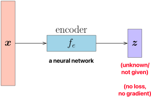
• Structure แบบนี้มัน Train ไม่ได้นะ (using Gradient Descent อะ) แล้วทำไงดี?
  • เฉลย ต้องมี Decoder
• Since target outputs are not provided, we train this model by creating a decoder that accepts the encoded array $z$ and reconstructs the input array $x$:
  $\boxed{\boldsymbol{r} = f_d(\boldsymbol{z}) = f_d(f_e(\boldsymbol{x}))}$
  

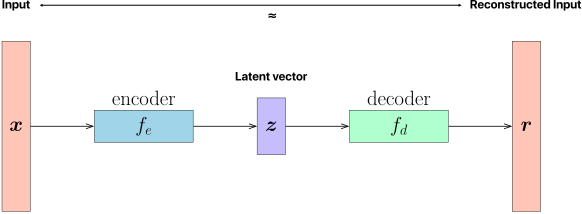
When $\vec{x}$ and $\vec{r}$ are approx. the same, $\vec{z}$ represents $\vec{x}$

• The encoder and decoder are connected and trained to reconstruct the input values - this complete system is called an autoencoder

14.2.1 Fully-connected Autoencoder

• Architecture: Input → Latent Vector → Reconstructed Input
  

$\boxed{r = g(W_2z + b_2) = g(W_2(g(W_1x + b_1)) + b_2)}$

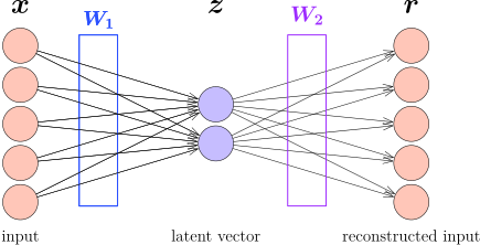
where:

• $x$ = input vector
• $z$ = latent vector (encoded representation)
• $r$ = reconstructed input
• $W_1, b_1$ = encoder weights and biases
• $W_2, b_2$ = decoder weights and biases
• $g$ = activation function

Loss Function

• Mean Squared Error (MSE) Loss:

$\boxed{L(x, r) = \frac{1}{m}\|x - r\|_2^2 = \frac{1}{m}\sum_{i=1}^{m}(x_i - r_i)^2}$
$m=\text{len}(\vec{x})$

• Binary Cross Entropy: Can be used when $0 \leq x_i \leq 1$ for all $i = 1, \ldots, m$

  • Using sigmoid activation function

• After training is complete, the decoder can be removed and only the encoder is used for feature extraction

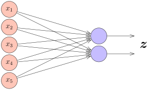
Relationship to PCA

• When the activation function is set to the linear function, this autoencoder works almost identically to Principal Component Analysis (PCA) technique
• Important difference: The encoder extracted from an autoencoder does not guarantee orthogonal components

PCA is like organizing your closet by color and type in perfectly perpendicular sections, while an autoencoder organizes it in whatever way makes sense, which might not be perfectly aligned.

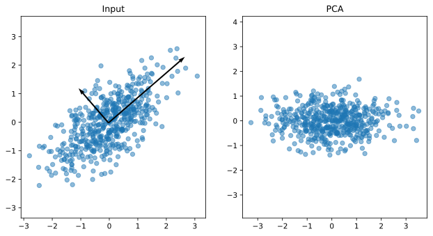
จะไม่ทำให้ดู ไม่ออกสอบแน่นอน

Techinique การทำ data analytics หาแกนหลักของข้อมูล ดูการตามกระจายของข้อมูล (คำนวณจากพวก covariance, ทิศไหนข้อมูลการกระจายมากที่สุด) → เราจึงลด Dimension ของมันได้ (ดูอะไรที่สำคัญที่สุด)

Example 14.1

Given:

• Input vector $x = [2, -1, 1]^{\top}$
• Fully-connected autoencoder with 2 hidden units and linear activation function

Encoder:
$\boldsymbol{z} = \boldsymbol{W}_e \boldsymbol{x} + \boldsymbol{b}_e$

where $W_e = \begin{bmatrix} 1 & 0 & -1 \\ 0 & 1 & 1 \end{bmatrix}$, $b_e = \begin{bmatrix} 0 \\ 1 \end{bmatrix}$

Decoder:
$\boldsymbol{r} = \boldsymbol{W}_d \boldsymbol{z} + \boldsymbol{b}_d$

where $W_d = \begin{bmatrix} 1 & 1 \\ 2 & 0 \\ 0 & 1 \end{bmatrix}$, $b_d = \begin{bmatrix} 0 \\ 0 \\ 1 \end{bmatrix}$

Task: Calculate the latent vector $\boldsymbol{z}$, reconstructed vector $\boldsymbol{r}$, and MSE loss between $\boldsymbol{x}$ and $\boldsymbol{r}$.

Solution:

1. Calculate latent vector $\boldsymbol{z}$:
   $z = W_e x + b_e = \begin{bmatrix} 1 & 0 & -1 \\ 0 & 1 & 1 \end{bmatrix} \begin{bmatrix} 2 \\ -1 \\ 1 \end{bmatrix} + \begin{bmatrix} 0 \\ 1 \end{bmatrix}$
   $z = \begin{bmatrix} 2(1) + (-1)(0) + 1(-1) \\ 2(0) + (-1)(1) + 1(1) \end{bmatrix} + \begin{bmatrix} 0 \\ 1 \end{bmatrix}$
   $z = \begin{bmatrix} 1 \\ 0 \end{bmatrix} + \begin{bmatrix} 0 \\ 1 \end{bmatrix} = \begin{bmatrix} 1 \\ 1 \end{bmatrix}$
   (New representation of $x$)
2. Calculate reconstructed vector $\boldsymbol{r}$:
   $r = W_d z + b_d = \begin{bmatrix} 1 & 1 \\ 2 & 0 \\ 0 & 1 \end{bmatrix} \begin{bmatrix} 1 \\ 1 \end{bmatrix} + \begin{bmatrix} 0 \\ 0 \\ 1 \end{bmatrix}$
   $r = \begin{bmatrix} 2 \\ 2 \\ 1 \end{bmatrix} + \begin{bmatrix} 0 \\ 0 \\ 1 \end{bmatrix} = \begin{bmatrix} 2 \\ 2 \\ 2 \end{bmatrix}$
   (Reconstruct of $x$)
3. Calculate MSE loss:
   $L_{\text{mse}}(x, r) =\frac{1}{m}\|\vec{x}-\vec{r}\|_2^2= \frac{1}{3}\sum_{i=1}^{3}(x_i - r_i)^2 = \frac{1}{3}[(2-2)^2 + (-1-2)^2 + (1-2)^2]$
   $L(x, r) = \frac{1}{3}[0 + 9 + 1] = \frac{10}{3} \approx 3.33$
   (แต่ $x$ ที่ reconstruct ก็ไม่ได้ดีขนาดนั้น ดังนั้น คำนวณหา Loss)

Multiple Hidden Layers

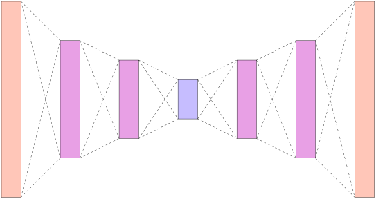
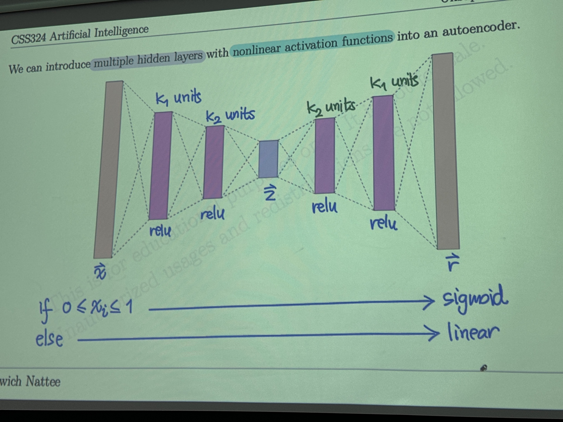
• We can introduce multiple hidden layers with nonlinear activation functions into an autoencoder
• This allows the autoencoder to learn more complex, non-linear representations

Example 14.2: MNIST Autoencoder

Given:

• MNIST dataset (handwritten digits)
• Encoder with 4 layers: 256, 128, 64, and 32 units
• Latent vector $z$ has 32 elements

Task: Fill in the decoder architecture

Layer Type	Units	Activation Function
Input	784	-
Fully Connected Later (Encoder)	256	relu
Fully Connected Later (Encoder)	128	relu
Fully Connected Later (Encoder)	64	relu
Fully Connected Later (Encoder)	32	relu
Fully Connected Later (Encoder)	64	relu
Fully Connected Later (Encoder)	128	relu
Fully Connected Later (Encoder)	256	relu
Fully Connected Later (Encoder)	784	sigmoid

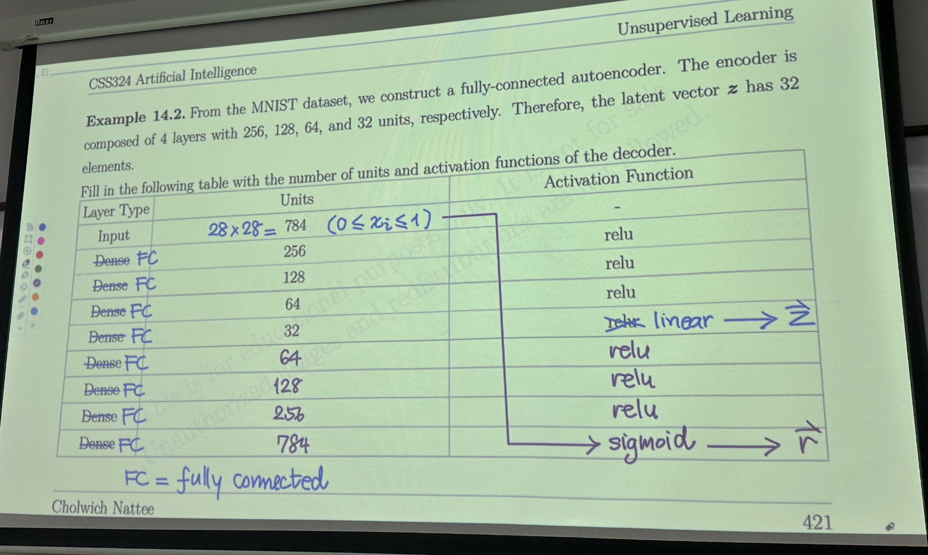The decoder mirrors the encoder architecture but in reverse, like unfolding an origami creation back to a flat sheet.

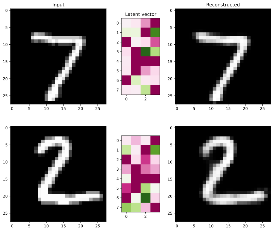
14.2.2 Convolutional Autoencoder

• Convolutional autoencoder includes at least one convolutional layer
• Each layer in the decoding part needs to increase size of its input array to reconstruct the input
• Two main techniques for upsampling:
  1. Transposed Convolution
  2. Upsampling + Convolution

Transposed Convolution

Algorithm:

Given an input array with shape $n_h \times n_w$ and a kernel with shape $k_h \times k_w$:

1. Create $n_h \cdot n_w$ intermediate arrays with shape $(n_h + k_h - 1) \times (n_w + k_w - 1)$, initialize all elements to zeros
2. Multiply each element of the input array with the kernel
3. Replace a portion of an intermediate array with the multiplication result
4. Sum all intermediate arrays to create the output array

Think of transposed convolution as the opposite of regular convolution - instead of shrinking the image, you're expanding it by "painting" each input value across a larger canvas.

Example 14.3: Transposed Convolution

Given:

• Input array: $\begin{bmatrix} 2 & 0 \\ 5 & 1 \end{bmatrix}$
• Kernel: $\begin{bmatrix} 1 & 2 \\ 2 & 3 \end{bmatrix}$

Process:

For each element in input, multiply by kernel and place in output:

1. $2 \cdot \begin{bmatrix} 1 & 2 \\ 2 & 3 \end{bmatrix} = \begin{bmatrix} 2 & 4 \\ 4 & 6 \end{bmatrix}$ (top-left)
2. $0 \cdot \begin{bmatrix} 1 & 2 \\ 2 & 3 \end{bmatrix} = \begin{bmatrix} 0 & 0 \\ 0 & 0 \end{bmatrix}$ (top-right)
3. $5 \cdot \begin{bmatrix} 1 & 2 \\ 2 & 3 \end{bmatrix} = \begin{bmatrix} 5 & 10 \\ 10 & 15 \end{bmatrix}$ (bottom-left)
4. $1 \cdot \begin{bmatrix} 1 & 2 \\ 2 & 3 \end{bmatrix} = \begin{bmatrix} 1 & 2 \\ 2 & 3 \end{bmatrix}$ (bottom-right)

Sum all overlapping regions:

$\text{Output} = \begin{bmatrix} 2 & 4 & 0 \\ 9 & 17 & 2 \\ 10 & 17 & 3 \end{bmatrix}$

Example 14.4

Given:

• Input: $x = \begin{bmatrix} 1 & 2 \\ 2 & 1 \end{bmatrix}$
• Kernel: $k = \begin{bmatrix} 1 & 2 & 3 \\ 3 & 1 & 2 \\ 2 & 1 & 3 \end{bmatrix}$

Task: Compute the output of transposed convolution

[Left for student to complete]

Upsampling

• Upsampling conducts the reverse of a pooling operation
• When performing upsampling on a 2D array with size $s_h \times s_w$:
  • Rows and columns are repeated by $s_h$ and $s_w$ respectively

Example: $2 \times 2$ upsampling

$\begin{bmatrix} 1 & 2 \\ 3 & 4 \end{bmatrix} \xrightarrow{\text{upsample } 2\times2} \begin{bmatrix} 1 & 1 & 2 & 2 \\ 1 & 1 & 2 & 2 \\ 3 & 3 & 4 & 4 \\ 3 & 3 & 4 & 4 \end{bmatrix}$

Upsampling is like taking a pixelated image and making it bigger by duplicating each pixel - simple but effective for increasing size.

• Alternative approach: A combination of upsampling and convolutional layers can be used in place of transposed convolutional layer

14.2.3 Denoise Autoencoder

Training Process:

1. Add noise to the input
2. Train the autoencoder using the original input as the target

• This type of autoencoder is called denoise autoencoder
• Benefits:
  • Makes the autoencoder more robust to noise
  • Improves the performance of dimensionality reduction

Like learning to read messy handwriting - the autoencoder becomes better at extracting the core features by learning to ignore the noise.

\usepackage{tikz, amsmath, amssymb}
\usetikzlibrary{arrows.meta, positioning, shapes}
\begin{document}
\begin{tikzpicture}[node distance=2.5cm, >=Stealth, thick]
% Nodes
\node (clean) {Clean\\Image};
\node[right=of clean] (noisy) {Noisy\\Image};
\node[draw, rectangle, fill=cyan!30, right=of noisy, minimum height=1.5cm] (encoder) {Encoder};
\node[draw, rectangle, fill=green!30, right=of encoder, minimum height=1.5cm] (decoder) {Decoder};
\node[right=of decoder] (output) {Reconstructed\\Clean Image};
 
% Arrows
\draw[->] (clean) -- node[above] {Add noise} (noisy);
\draw[->] (noisy) -- (encoder);
\draw[->] (encoder) -- (decoder);
\draw[->] (decoder) -- (output);
\draw[->, dashed, red] (clean) to[bend left=45] node[above] {Target} (output);
\end{tikzpicture}
\end{document}

[Image: Shows progression from clean digit → noisy digit → encoder → decoder → reconstructed clean digit]

14.3 Generative Adversarial Network (GAN)

Overview

• GAN (Generative Adversarial Network), proposed by Goodfellow et al. in 2014
• A generative model originally designed to generate new data
• Composed of two parts:

1. Generator ($G$): Learns to generate fake data
2. Discriminator ($D$): Learns to determine whether an example is real or fake

\usepackage{tikz, amsmath, amssymb}
\usetikzlibrary{arrows.meta, positioning, shapes}
\begin{document}
\begin{tikzpicture}[node distance=2.5cm, >=Stealth, thick]
% Nodes
\node[draw, rectangle, fill=gray!40] (noise) {Random\\Noise\\$z$};
\node[draw, rectangle, fill=blue!40, right=of noise, minimum height=1.5cm, minimum width=2cm] (generator) {Generator\\$G$};
\node[draw, rectangle, fill=red!30, below right=1cm and 1cm of generator] (fake) {Generated\\Example\\$G(z)$};
\node[draw, rectangle, fill=green!30, above right=1cm and 1cm of generator] (real) {Real\\Example\\$x$};
\node[draw, rectangle, fill=magenta!40, right=3cm of generator, minimum height=2cm, minimum width=2cm] (discriminator) {Discriminator\\$D$};
\node[right=of discriminator] (output) {$D(x)$ or\\$D(G(z))$};
 
% Arrows
\draw[->] (noise) -- (generator);
\draw[->] (generator) -- (fake);
\draw[->] (fake) -- (discriminator);
\draw[->] (real) -- (discriminator);
\draw[->] (discriminator) -- (output);
\end{tikzpicture}
\end{document}

Think of GANs like an art forger (generator) trying to fool an art expert (discriminator). As the expert gets better at detecting fakes, the forger improves their technique, and vice versa.

Minimax Loss Function

$\boxed{V(\theta_d, \theta_g) = \mathbb{E}_x[\log D(x)] + \mathbb{E}_z[\log(1 - D(G(z)))]}$
Where:

• $x$ = real example
• $z$ = noise (random input)
• $D(x)$ = probability that $x$ is real (estimated by discriminator)
• $G(z)$ = example generated from noise $z$
• $D(G(z))$ = probability that generated example is real
• $\mathbb{E}_x$ = expected value over all real examples
• $\mathbb{E}_z$ = expected value over all random noises

Training Objective:

$\boxed{\min_G \max_D V(\theta_d, \theta_g)}$

• Discriminator: Trained to maximize the loss
• Generator: Trained to minimize the loss

Training Algorithm

Algorithm 1: Minibatch stochastic gradient descent training of GANs

Hyperparameter: $k$ = number of discriminator steps per generator step (often $k=1$)

For each training iteration:

Phase 1: Train Discriminator (repeat $k$ times)

• Sample minibatch of $m$ noise samples $\{z^{(1)}, \ldots, z^{(m)}\}$ from noise prior $p_g(z)$

• Sample minibatch of $m$ examples $\{x^{(1)}, \ldots, x^{(m)}\}$ from data distribution $p_{data}(x)$

• Update discriminator by ascending its stochastic gradient:

  $\nabla_{\theta_d} \frac{1}{m}\sum_{i=1}^{m}[\log D(x^{(i)}) + \log(1 - D(G(z^{(i)})))]$

Phase 2: Train Generator

• Sample minibatch of $m$ noise samples $\{z^{(1)}, \ldots, z^{(m)}\}$ from noise prior $p_g(z)$

• Update generator by descending its stochastic gradient:

  $\nabla_{\theta_g} \frac{1}{m}\sum_{i=1}^{m}\log(1 - D(G(z^{(i)})))$

GAN Training Steps - Detailed

Step 1: Train the Discriminator

Freeze generator parameters

1. Create a minibatch of real data
2. Create a minibatch of noises and use generator to synthesize fake data
3. Use gradient ascent to update discriminator parameters to maximize $V(\theta_d, \theta_g)$:

$\text{maximize } \left[\frac{1}{n}\sum_{i=1}^{n}[\log(D(x^{[i]})) + \log(1 - D(G(z^{[i]})))]\right]$

Equivalently, use gradient descent to minimize negative log likelihood:

$\text{minimize } \left[-\frac{1}{n}\sum_{i=1}^{n}[\log(D(x^{[i]})) + \log(1 - D(G(z^{[i]})))]\right]$

Comparison to Binary Cross Entropy:

$\text{minimize } \left[-\frac{1}{n}\sum_{i=1}^{n}[y^{[i]}\log(\hat{y}) + (1-y)\log(1-\hat{y})]\right]$

Key Insight: Training discriminator to maximize $V(\theta_d, \theta_g)$ is equivalent to training with binary cross entropy where:

• Target = 1 for real data
• Target = 0 for generated/fake data

Step 2: Train the Generator

Freeze discriminator parameters

1. Create a minibatch of noises and use generator to synthesize fake data
2. Use gradient descent to update generator parameters to minimize $V(\theta_d, \theta_g)$:

$\text{minimize } \frac{1}{n}\sum_{i=1}^{n}[\log(1 - D(G(z^{[i]})))]$

Problem: At early training stage:

• Generator synthesizes data that doesn't look like real data
• Discriminator easily predicts generated data as fake with high confidence
• Causes vanishing gradient problem (error must propagate backward from discriminator to generator)

Solution: To avoid saturation, adjust training to:

$\text{maximize } \left[\frac{1}{n}\sum_{i=1}^{n}[\log(D(G(z^{[i]})))]\right]$

Equivalently:

$\text{minimize } \left[-\frac{1}{n}\sum_{i=1}^{n}[\log(D(G(z^{[i]})))]\right]$

This is equivalent to using binary cross entropy with target = 1

Effect: Generator is trained to maximize the probability of generated data being predicted as real

Instead of trying to make fake data "less fake," we train the generator to make fake data "more real" - this provides stronger gradients early in training.

GAN Training Visualization

[Image: Four stages (a-d) showing the evolution of GAN training]

Training Progress:

(a) Initial state:

• $p_g$ (generator distribution, green) differs from $p_{data}$ (real data, black dots)
• $D$ (discriminator, blue dashed) is partially accurate

(b) Discriminator training:

• In inner loop, $D$ is trained to discriminate samples from data
• Converges to $D^*(x) = \frac{p_{data}(x)}{p_{data}(x) + p_g(x)}$

(c) Generator update:

• After generator update, gradient of $D$ guides $G(z)$ to flow toward regions more likely to be classified as data

(d) Convergence:

• After several training steps, if $G$ and $D$ have enough capacity:
• Reach point where $p_g = p_{data}$
• Discriminator cannot differentiate: $D(x) = \frac{1}{2}$

Generated Samples

[Image: Examples of GAN-generated images]

Examples shown:

• a) MNIST digits (handwritten numbers)
• b) Face images
• c) Natural scenes
• d) Animals and objects

Rightmost column shows nearest training example (to verify not memorizing)

Vector Arithmetic in Latent Space

Concept: GANs learn meaningful latent representations that support vector arithmetic

Example:
$\text{man with glasses} - \text{man without glasses} + \text{woman without glasses} = \text{woman with glasses}$

[Image: Visual demonstration of vector arithmetic producing women with glasses]

The latent space learns abstract concepts like "glasses-ness" that can be added or subtracted from generated images, similar to how word embeddings work (king - man + woman = queen).

References

• Goodfellow et al. "Generative Adversarial Nets." Advances in Neural Information Processing Systems. 2014.
• Radford et al. "Unsupervised Representation Learning with Deep Convolutional Generative Adversarial Networks." ICLR 2016.

Summary

Key Concepts

Autoencoders:

• Learn compressed representations through reconstruction
• Encoder: $z = f_e(x)$
• Decoder: $r = f_d(z)$
• Loss: MSE or Binary Cross Entropy
• Variations: Fully-connected, Convolutional, Denoise

GANs:

• Two-player game: Generator vs Discriminator
• Generator creates fake data
• Discriminator distinguishes real from fake
• Minimax objective: $\min_G \max_D V(\theta_d, \theta_g)$
• Training alternates between improving D and G
• Converges when $p_g = p_{data}$