10.1 Training a Neural Network

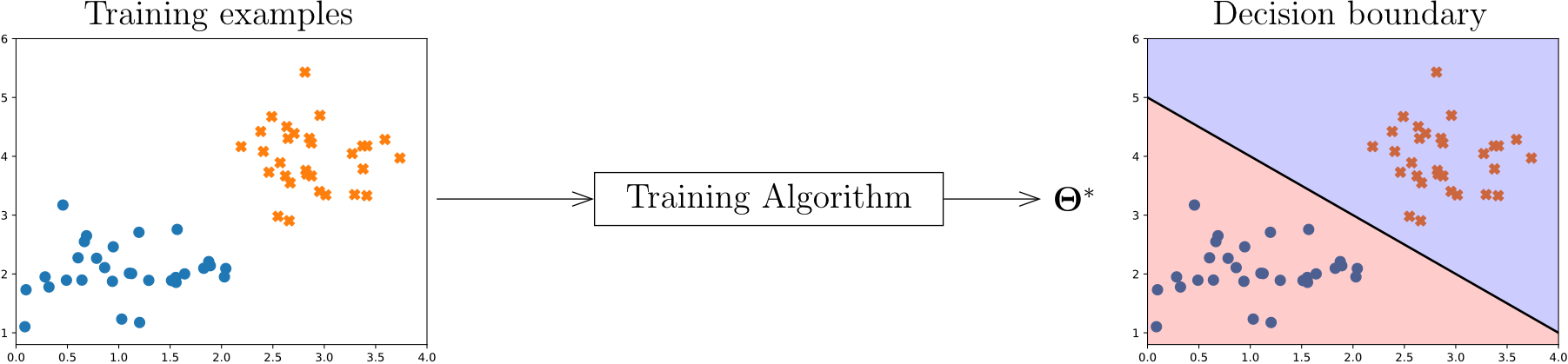
Training a neural network is a process to adjust its parameters based on a training set to ensure it correctly classifies the data.

$\boxed{\hat{y} = h(x; \theta)}$

where:

• $\theta$ is the set of parameters of the neural network
• $\theta = \{W^{[1]}, b^{[1]}, \ldots, W^{[L]}, b^{[L]}\}$

Analogy: Think of training a neural network like teaching a student. The training examples are like practice problems, and the training algorithm adjusts the "knowledge" (parameters) to help the network make better predictions, eventually finding the optimal decision boundary.

Visual representation:

• Training examples → Training Algorithm → $\Theta^*$ → Decision boundary

10.2 Training Set

To train a neural network, เราก็ต้องมี Training set ถูกป่าว

A training set is composed of pairs of an input vector and a target output.
$\boxed{D = \{(x_1, y_1), (x_2, y_2), (x_3, y_3), \ldots, (x_N, y_N)\}}$

where:

• Each $(x_i, y_i)$ is a labeled example, when $i \in [1, \ldots, N]$
• Each $x_i = [x_{i1} \quad x_{i2} \quad \ldots \quad x_{iM}]^{\top}$ is an input vector
• Each $y_i$ is a target output
• $N$ is the number of training examples
• $M$ is the number of features

Analogy: A training set is like a textbook with answers. Each example $(x_i, y_i)$ is a question-answer pair where $x_i$ is the question and $y_i$ is the correct answer.

Example 10.1

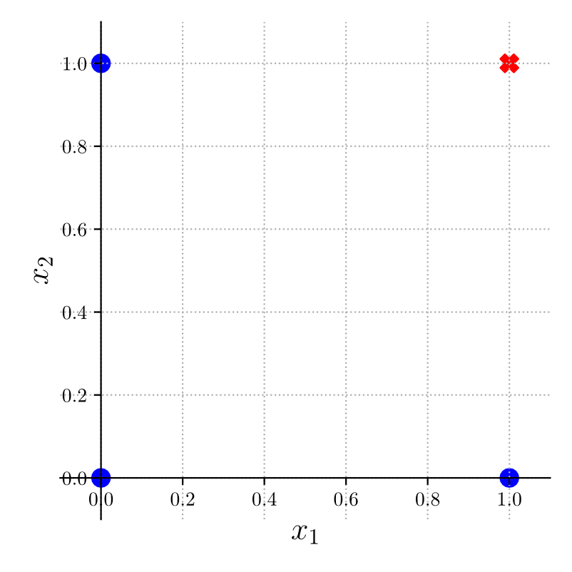
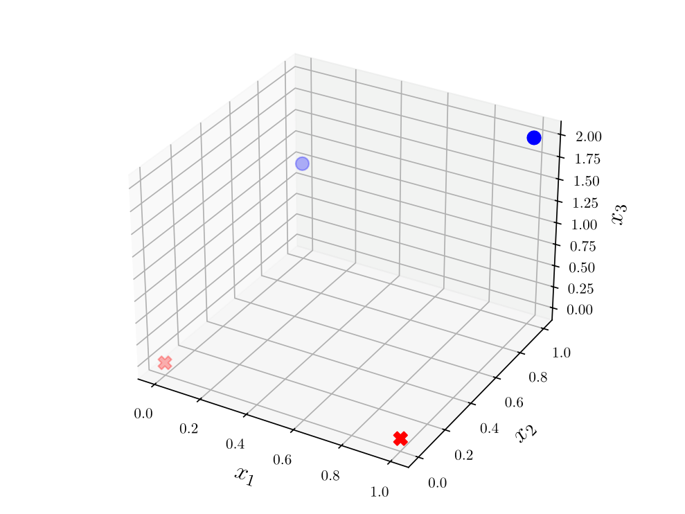
Write the training set visualized by the following plot.
Note: use 0 for ● and 1 for ×.

ก็แค่เขียนว่าแต่ละจุดคือตรงไหน แล้วก็ สีจะเป็นการบอก Output

Example 10.2

Write the training set visualized by the following plot.
Note: use 0 for ● and 1 for ×.

$N=4,M=3$

10.3 Gradient Descent

Key Points:

• Gradient descent is a common method to train a neural network
• It is an iterative optimization algorithm for finding the values of parameters of a function that minimizes a differentiable objective function (คล้าย ๆ กับ Chapter 5 - Local Search)
  • ต่างกันตรงที่ว่า Function ที่จะ Work กับ Gradient Descent ก็คือต้องเป็น Differentiable Function
• It works similarly to the hill-climbing algorithm but operates in a continuous space
  • ถ้าที่เราเรียนใน Chapter 5 - Local Search → Discrete Space
    • ก็คือมี Limit ในเรื่องของทางที่มันไปได้ (Up, Down, Left, Right)
    • ซึ่งมี Step Size เป็น 1 เท่านั้น
  • แต่ Gradient Descent เป็น continuous space ไปทางไหนก็ได้ 360 องศาเลยล่ะ
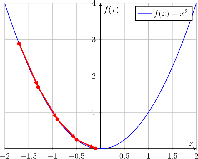
• It operates by updating the parameters in the direction of the negative gradient of the objective function, gradually moving towards a minimum

Update Rule

Given an objective function $J(\theta)$, the gradient descent algorithm updates the parameters $\theta$ iteratively as follows:
$\boxed{\theta \leftarrow \theta - \eta \nabla_\theta J(\theta)}$
where:

• $\eta$ is the step size or learning rate (a hyperparameter that controls the step size)
• $\nabla_\theta J(\theta)$ is the gradient of the objective function with respect to the parameters
  • Gradient = Direction นั่นแหละ

$\Huge\nabla_\theta J(\theta) = \begin{bmatrix} \frac{\partial J}{\partial \theta_1} \\ \frac{\partial J}{\partial \theta_2} \\ \vdots \\ \frac{\partial J}{\partial \theta_k} \end{bmatrix}$

Analogy: Imagine you're hiking down a mountain in fog. You can only see your immediate surroundings. Gradient descent is like taking small steps in the direction that slopes downward the most steeply. The learning rate $\eta$ controls how big each step is.

Visual Example

For example, given an objective function $f(x) = x^2$: (We want to find $x$ that makes $f(x)$ be the minimum)

• ตัวอย่าง
  • Let $\eta=0.1,x_0=-1.75$

In each iteration, the parameter $x$ is updated by:
$\boxed{x \leftarrow x - \eta \frac{d}{dx}f(x) = x - \eta(2x)}$

Update $x$ ใช้ Formula ด้านบน — จากข้างบนก็แปลว่า every iteration, we update $x$ by $x-\eta(2x)$

10.4 Training a Neural Network using Gradient Descent

ถ้าเราจะใช้ Gradient Descent ในการ Train Neural Network

To train a neural network using the gradient descent algorithm, we need an objective function $L(x_i,y_i;\theta) \quad \theta=\{w,b \dotso\}$ that:

• Represents how well the neural network is performing
  • ก็แค่ compare $y_i$ (target output) กับ $\hat{y_i}$ (predicted output) ว่ามันต่างกันแค่ไหน
• Includes the weights and the bias of the neural network as its parameters

The gradient descent algorithm can then be used to iteratively update the weights and bias of the neural network to minimize the objective function. Thus, the neural network learns to make accurate predictions on the training set.

10.5 Loss Function

Objective Function ที่ใช้กับ 10.4 Training a Neural Network using Gradient Descent นั่นเอง

A loss function is a mathematical function that quantifies the difference between the predicted output of a model ($\hat{y_i}$) and the actual target output ($y_i$). It measures how well the model is performing on a given dataset.

The choice of loss function depends on the specific task and the type of output the model is producing.

Common Loss Functions

1. Squared Error Loss Function

Quantifies the difference between target and predicted outputs. Commonly used for ==regression tasks.==

• Regression task → $y_i\in\mathbb{R}$

$\Huge\boxed{L_{se}(x_i, y_i; w, b) = \|\hat{y}_i - y_i\|^2}$
Properties:

• When $\hat{y}_i$ is close to $y_i$, $L_{se}$ is small
• When $\hat{y}_i$ is far from $y_i$, $L_{se}$ is large

We need to square because we want the error (loss) to be positive, ถ้ามีบวกบ้าง มีลบบ้าง สรุปคือเราเอามา Sum กันได้ 0 งงเลยล่ะ Loss เป็นศูนย์แต่จริง ๆ แล้วพังเยอะ

Analogy: Squared error is like measuring how far your dart is from the bullseye. The further away, the bigger the penalty, and it squares the distance to punish larger errors more heavily.

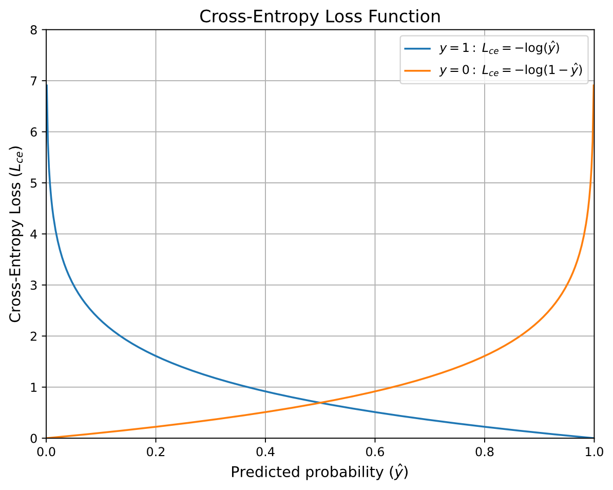
2. Cross-Entropy Loss Function

Commonly used for ==classification tasks==, especially with sigmoid units.

• Classification task → $y_i\in\{0,1\}$
  $\Huge\boxed{L_{ce}(x_i, y_i; w, b) = -[y_i \log(\hat{y}_i) + (1 - y_i) \log(1 - \hat{y}_i)]}$

Properties:

• When $y_i = 1$: $\boxed{L_{ce} = -\log(\hat{y}_i)}$
  • As $\hat{y}_i$ approaches 1, $L_{ce}$ approaches 0
  • As $\hat{y}_i$ approaches 0, $L_{ce}$ tends to infinity
• When $y_i = 0$: $\boxed{L_{ce} = -\log(1 - \hat{y}_i)}$
  • As $\hat{y}_i$ approaches 0, $L_{ce}$ approaches 0
  • As $\hat{y}_i$ approaches 1, $L_{ce}$ tends to infinity

Analogy: Cross-entropy loss is like a confidence penalty. If the model is very confident (prediction close to 1) but wrong (actual is 0), the penalty shoots up dramatically. It rewards confident correct predictions and heavily punishes confident wrong predictions.

Example 10.3

When $y_i = 1$ and $\hat{y}_i = 0.82$, calculate the squared error loss and the cross-entropy loss.

Squared Error Loss:
$L_{se} = (0.82 - 1)^2 = 0.0324$

Cross-Entropy Loss:
$L_{ce} = -[1 \cdot \log(0.82) + 0 \cdot \log(1-0.82)] = -\log(0.82) \approx 0.198$

10.6 Batch Gradient Descent

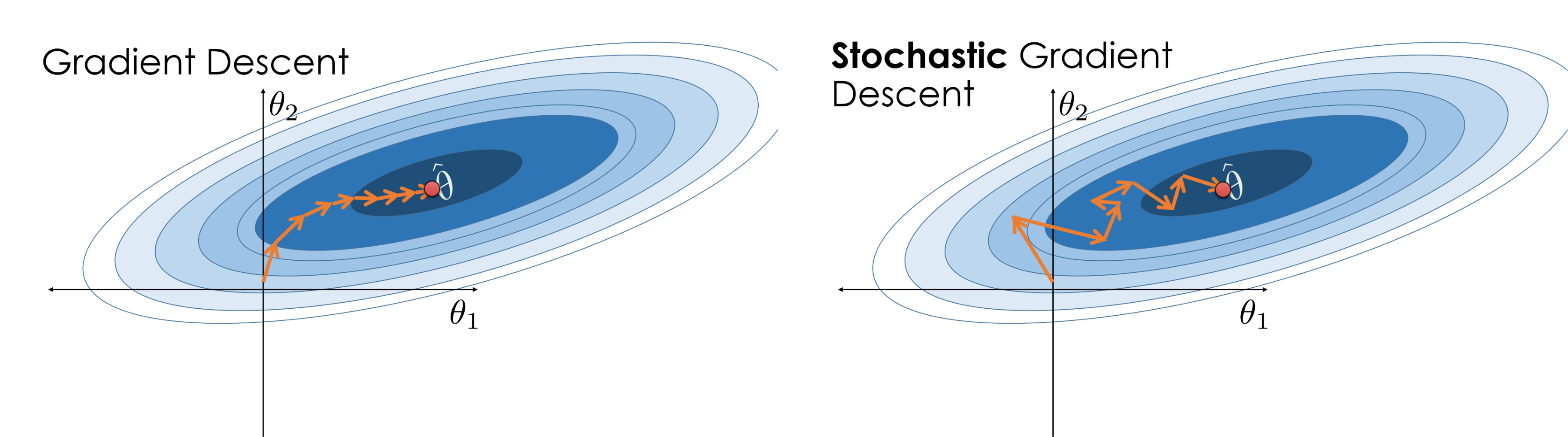
Batch gradient descent is a variant that uses the entire training set to compute gradients in each iteration.

Algorithm

Input: A training set $D = \{(x_i, y_i)\}_{i=1}^{N}$

1. Initialize model parameters $\theta$ (e.g., weights and biases) randomly or with small values
2. for $e = 1$ to $E$ (epochs/training iterations):
   1. for $(x_i, y_i) \in \mathcal{D}$:
      1. Compute predicted output: $\hat{y}_i = h(x_i; \theta)$
      2. Compute gradient $\nabla_\theta L(x_i, y_i; \theta)$
   2. Compute average gradient:
      $\nabla_\theta L(\theta) = \frac{1}{N}\sum_{i=1}^{N} \nabla_\theta L(x_i, y_i; \theta)$
   3. Update model parameters:
      $\theta \leftarrow \theta - \eta \nabla_\theta L(\theta)$

Analogy: Batch gradient descent is like a teacher grading all homework assignments before deciding what to teach next. You look at everyone's mistakes, find the average problem areas, and adjust your teaching accordingly.

10.7 Stochastic Gradient Descent

แทนที่จะเป็นแบบข้างบนมาอย่างเยอะ เราแบ่งเป็น Mini-batch แล้ว compute gradient ของแต่ละ Mini-batch

Stochastic gradient descent (SGD) is a variant of the gradient descent algorithm that updates the model parameters using the gradient computed from a small, randomly selected subset of the training data (minibatch) at each iteration.

Algorithm

Input: A training set $D = \{(x_i, y_i)\}_{i=1}^{N}$, minibatch size $B$

1. Initialize model parameters $\theta$ (e.g., weights and biases) randomly or with small values
2. for $e = 1$ to $E$ (epochs):
   1. Split $\mathcal{D}$ into minibatches of size $B$: $\{\mathcal{B_1}, \mathcal{B_2}, \ldots, \mathcal{B}_T\}$ where $T = \lceil \frac{N}{B} \rceil$
   2. for $t = 1$ to $T$:
      1. for $(x_i, y_i)$ in $\mathcal{B}_t$:
         1. Compute predicted output: $\hat{y}_i = h(x_i; \theta)$
         2. Compute gradient $\nabla_\theta L(x_i, y_i; \theta)$
      2. Compute minibatch-level gradient:
         $\nabla_\theta L_B(\theta) = \frac{1}{B}\sum_{i=1}^{B} \nabla_\theta L(x_i, y_i; \theta)$
      3. Update model parameters:
         $\theta \leftarrow \theta - \eta \nabla_\theta L_B(\theta)$
         Number of updates = $T\times E$

Comparison between Batch GD and SGD

แค่ต่างกันตรง Data ที่เอาไว้ Calculate Gradient นั่นแหละ

(Batch) GD:

• Uses the entire dataset to compute gradients
• ==More stable convergence== but can be slow for large datasets

SGD:

• Uses a single sample (or minibatch) to compute gradients
• Faster updates and can escape local minima, but more noisy
  • Escape local minima ได้ด้วยเพราะมัน Zig-zag 55555
  • เดี๋ยวนี้ใช้อันนี้กันหมด เพราะว่ามันดีกว่า in terms of memory management or something

Analogy: If Batch GD is like surveying everyone in a city before making a decision, SGD is like asking a random sample of people and making quicker (but noisier) decisions. SGD's path is more zigzagged but often reaches the goal faster.

Example 10.4

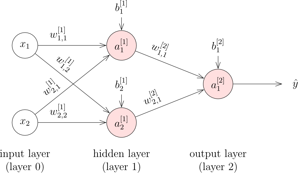
Given the MLP for the XOR function below, use the SGD algorithm to update the weights and biases using a minibatch size of 2: $B_1 = \{([0, 0]^T, 0), ([1, 0]^T, 1)\}$, learning rate $\eta = 0.1$, and the cross entropy loss function.

Using the cross-entropy loss function:
$L_{ce}(x_i, y_i; \theta) = -[y_i \log(\hat{y}_i) + (1-y_i)\log(1-\hat{y}_i)]$

Initial Parameters

$W^{[1]} = \begin{bmatrix} 0.1 & 0.2 \\ 0.3 & 0.1 \end{bmatrix}, \quad b^{[1]} = \begin{bmatrix} -0.01 \\ 0.02 \end{bmatrix}$
$W^{[2]} = \begin{bmatrix} 0.05 & 0.05 \end{bmatrix}, \quad b^{[2]} = -0.2$

Step 1:

Process first example $x_i = [0, 0]^T$, $y_i = 0$

Forward pass:

$z_i^{[1]} = W^{[1]}x_i + b^{[1]} = \begin{bmatrix} 0.1 & 0.2 \\ 0.3 & 0.1 \end{bmatrix} \begin{bmatrix} 0 \\ 0 \end{bmatrix} + \begin{bmatrix} -0.01 \\ 0.02 \end{bmatrix} = \begin{bmatrix} -0.01 \\ 0.02 \end{bmatrix}$
$a_i^{[1]} = \sigma(z_i^{[1]}) = \begin{bmatrix} \sigma(-0.01) \\ \sigma(0.02) \end{bmatrix} = \begin{bmatrix} 0.4975 \\ 0.5050 \end{bmatrix}$
$z_i^{[2]} = W^{[2]}a_i^{[1]} + b^{[2]} = [0.05 \quad 0.05] \begin{bmatrix} 0.4975 \\ 0.5050 \end{bmatrix} + (-0.2) = -0.1499$
$a_i^{[2]} = \sigma(z_i^{[2]}) = \sigma(-0.1499) = 0.4626$
$\hat{y}_i = a_i^{[2]} = 0.4626$

Gradient computation for Layer 2:
For $w_{1,1}^{[2]}$: (To update we need to compute $\frac{\partial L_{ce,i}}{\partial w_{1,1}^{[2]}}$ first)

$\frac{\partial L_{ce,i}}{\partial w_{1,1}^{[2]}} = \left(\frac{\partial L_{ce,i}}{\partial \hat{y}_i}\right)\left(\frac{\partial \hat{y}_i}{\partial z_{i,1}^{[2]}}\right)\left(\frac{\partial z_{i,1}^{[2]}}{\partial w_{1,1}^{[2]}}\right)$

Through chain rule derivation:
$\boxed{\frac{\partial L_{ce,i}}{\partial w_{1,1}^{[2]}} = (\hat{y}_i - y_i)a_{i,1}^{[1]}}$
Similarly:
$\boxed{\frac{\partial L_{ce,i}}{\partial w_{2,1}^{[2]}} = (\hat{y}_i - y_i)a_{i,2}^{[1]}}$
$\boxed{\frac{\partial L_{ce,i}}{\partial b^{[2]}} = (\hat{y}_i - y_i)}$
Gradient computation for Layer 1:
For $w_{1,1}^{[1]}$:
$\frac{\partial L_{ce,i}}{\partial w_{1,1}^{[1]}} = \left(\frac{\partial L_{ce,i}}{\partial \hat{y}_i}\right)\left(\frac{\partial \hat{y}_i}{\partial z_{i,1}^{[2]}}\right)\left(\frac{\partial z_{i,1}^{[2]}}{\partial a_{i,1}^{[1]}}\right)\left(\frac{\partial a_{i,1}^{[1]}}{\partial z_{i,1}^{[1]}}\right)\left(\frac{\partial z_{i,1}^{[1]}}{\partial w_{1,1}^{[1]}}\right)$
$\boxed{= (\hat{y}_i - y_i)(1)(w_{1,1}^{[2]})\Big(a_{i,1}^{[1]}(1-a_{i,1}^{[1]})\Big)(x_{i,1})}$

Similarly for other weights and biases in Layer 1.

Computed gradients for first example:

แก้สมการรอบเดียว แค่เปลี่ยนตัวแปร สำหรับ Weight อื่น ๆ อะนะ

Layer 2:

• $\frac{\partial L_{ce,1}}{\partial w_{1,1}^{[2]}} = (0.4626 - 0)(0.4975) = 0.2301$
• $\frac{\partial L_{ce,1}}{\partial w_{2,1}^{[2]}} = (0.4626 - 0)(0.5050) = 0.2336$
• $\frac{\partial L_{ce,1}}{\partial b^{[2]}} = (0.4626 - 0)(1) = 0.4626$

Layer 1 (Hidden layer):

• $\frac{\partial L_{ce,1}}{\partial w_{1,1}^{[1]}} = 0$ (since $x_{i,1} = 0$)
• $\frac{\partial L_{ce,1}}{\partial w_{1,2}^{[1]}} = 0$ (since $x_{i,2} = 0$)
• $\frac{\partial L_{ce,1}}{\partial b_1^{[1]}} = 0.0058$
• $\frac{\partial L_{ce,1}}{\partial w_{2,1}^{[1]}} = 0$ (since $x_{i,1} = 0$)
• $\frac{\partial L_{ce,1}}{\partial w_{2,2}^{[1]}} = 0$ (since $x_{i,2} = 0$)
• $\frac{\partial L_{ce,1}}{\partial b_2^{[1]}} = 0.0058$

Step 2:

Process second example $x_i = [1, 0]^T$, $y_i = 1$ from $\mathcal{B}_1$

Forward pass:

$z_i^{[1]} = \begin{bmatrix} 0.09 \\ 0.32 \end{bmatrix}, \quad a_i^{[1]} = \begin{bmatrix} 0.5225 \\ 0.5793 \end{bmatrix}$

$z_i^{[2]} = -0.1449, \quad a_i^{[2]} = 0.4638$

$\hat{y}_i = 0.4638$

Computed gradients for second example:
Layer 2:

• $\frac{\partial L_{ce,2}}{\partial w_{1,1}^{[2]}} = (0.4638 - 1)(0.5225) = -0.2802$
• $\frac{\partial L_{ce,2}}{\partial w_{2,1}^{[2]}} = (0.4638 - 1)(0.5793) = -0.3106$
• $\frac{\partial L_{ce,2}}{\partial b^{[2]}} = (0.4638 - 1)(1) = -0.5362$

Layer 1:

• $\frac{\partial L_{ce,2}}{\partial w_{1,1}^{[1]}} = -0.0067$
• $\frac{\partial L_{ce,2}}{\partial w_{1,2}^{[1]}} = 0$
• $\frac{\partial L_{ce,2}}{\partial b_1^{[1]}} = -0.0067$
• $\frac{\partial L_{ce,2}}{\partial w_{2,1}^{[1]}} = -0.0065$
• $\frac{\partial L_{ce,2}}{\partial w_{2,2}^{[1]}} = 0$
• $\frac{\partial L_{ce,2}}{\partial b_2^{[1]}} = -0.0065$

Step 3:

Compute minibatch-level gradient

Layer 2:

• $\frac{\partial L_{ce,\mathcal{B}}}{\partial w_{1,1}^{[2]}} = \frac{1}{2}(0.2301 - 0.2802) = -0.0251$
• $\frac{\partial L_{ce,\mathcal{B}}}{\partial w_{2,1}^{[2]}} = \frac{1}{2}(0.2336 - 0.3106) = -0.0385$
• $\frac{\partial L_{ce,\mathcal{B}}}{\partial b^{[2]}} = \frac{1}{2}(0.4626 - 0.5362) = -0.0368$

Layer 1:

• $\frac{\partial L_{ce,\mathcal{B}}}{\partial w_{1,1}^{[1]}} = \frac{1}{2}(0 - 0.0067) = -0.0034$
• $\frac{\partial L_{ce,\mathcal{B}}}{\partial w_{1,2}^{[1]}} = \frac{1}{2}(0 + 0) = 0$
• $\frac{\partial L_{ce,\mathcal{B}}}{\partial b_1^{[1]}} = \frac{1}{2}(0.0058 - 0.0067) = -0.0005$
• $\frac{\partial L_{ce,\mathcal{B}}}{\partial w_{2,1}^{[1]}} = \frac{1}{2}(0 - 0.0065) = -0.0032$
• $\frac{\partial L_{ce,\mathcal{B}}}{\partial w_{2,2}^{[1]}} = \frac{1}{2}(0 + 0) = 0$
• $\frac{\partial L_{ce,\mathcal{B}}}{\partial b_2^{[1]}} = \frac{1}{2}(0.0058 - 0.0065) = -0.0004$

Step 4:

Update model parameters using $\eta = 0.1$

Layer 2:

• $w_{1,1}^{[2]} \leftarrow 0.05 - 0.1(-0.0251) = 0.0525$
• $w_{2,1}^{[2]} \leftarrow 0.05 - 0.1(-0.0385) = 0.0539$
• $b^{[2]} \leftarrow -0.2 - 0.1(-0.0368) = -0.1963$

Layer 1:

• $w_{1,1}^{[1]} \leftarrow 0.1 - 0.1(-0.0034) = 0.1003$
• $w_{1,2}^{[1]} \leftarrow 0.2 - 0.1(0) = 0.2$
• $b_1^{[1]} \leftarrow -0.01 - 0.1(-0.0005) = -0.0099$
• $w_{2,1}^{[1]} \leftarrow 0.3 - 0.1(-0.0032) = 0.3003$
• $w_{2,2}^{[1]} \leftarrow 0.1 - 0.1(0) = 0.1$
• $b_2^{[1]} \leftarrow 0.02 - 0.1(-0.0004) = 0.0200$

Example 10.5

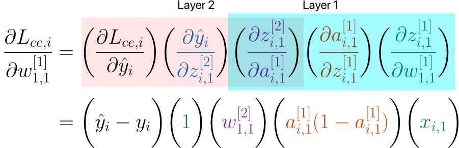
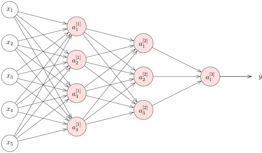
Given an MLP with $W^{[1]} \in \mathbb{R}^{4 \times 5}$, $b^{[1]} \in \mathbb{R}^4$, $W^{[2]} \in \mathbb{R}^{3 \times 4}$, $b^{[2]} \in \mathbb{R}^3$, $W^{[3]} \in \mathbb{R}^{1 \times 3}$, and $b^{[3]} \in \mathbb{R}$, write the product of partial derivatives using the chain rule to compute:

• $\frac{\partial L_{ce,i}}{\partial w_{1,1}^{[3]}}$
• $\frac{\partial L_{ce,i}}{\partial b_2^{[2]}}$
• $\frac{\partial L_{ce,i}}{\partial w_{5,2}^{[1]}}$

Note: all neurons use the sigmoid activation function, and the loss function is cross-entropy loss.

Solutions:
$\frac{\partial L_{ce,i}}{\partial w_{1,1}^{[3]}} = \left(\frac{\partial L_{ce,i}}{\partial \hat{y}_i}\right)\left(\frac{\partial \hat{y}_i}{\partial z_{i,1}^{[3]}}\right)\left(\frac{\partial z_{i,1}^{[3]}}{\partial w_{1,1}^{[3]}}\right)$
$\frac{\partial L_{ce,i}}{\partial b_2^{[2]}} = \left(\frac{\partial L_{ce,i}}{\partial \hat{y}_i}\right)\left(\frac{\partial \hat{y}_i}{\partial z_{i,1}^{[3]}}\right)\left(\frac{\partial z_{i,1}^{[3]}}{\partial a_{i,2}^{[2]}}\right)\left(\frac{\partial a_{i,2}^{[2]}}{\partial z_{i,2}^{[2]}}\right)\left(\frac{\partial z_{i,2}^{[2]}}{\partial b_2^{[2]}}\right)$

10.8 Optimizers

Optimizers are algorithms or methods used to adjust the parameters of a neural network during training to minimize the loss function.

Adam (Adaptive Moment Estimation)

ช่วยให้ Converge faster than 10.7 Stochastic Gradient Descent เฉย ๆ

Adam is an optimization algorithm that combines the benefits of two other popular optimizers: AdaGrad and RMSProp. It computes adaptive learning rates for each parameter by maintaining running averages of both the gradients and their squared values.

Update Rules

Given parameters $w$, gradient $g_t$, and learning rate $\eta$, instead of updating parameters using the raw gradient:
$w_t = w_{t-1} - \eta g_t$

The Adam update rules are:
$\boxed{m_t = \beta_1 m_{t-1} + (1-\beta_1)g_t}$ (First moment estimate)
$\boxed{v_t = \beta_2 v_{t-1} + (1-\beta_2)g_t^2}$ (Second moment estimate)
$\boxed{\hat{m}_t = \frac{m_t}{1-\beta_1^t}}$ (Bias-corrected first moment)
$\boxed{\hat{v}_t = \frac{v_t}{1-\beta_2^t}}$ (Bias-corrected second moment)
$\boxed{w_t = w_{t-1} - \eta \frac{\hat{m}_t}{\sqrt{\hat{v}_t} + \epsilon}}$ (Parameter update)

where:

• $m_t$ is the first moment estimate (mean of gradients)
• $v_t$ is the second moment estimate (uncentered variance of gradients)
• $\hat{m}_t$ and $\hat{v}_t$ are bias-corrected estimates of $m_t$ and $v_t$, respectively
  • Aims to correct the initialization bias towards zero, especially during initial time steps
• $\beta_1$ and $\beta_2$ are hyperparameters that control the decay rates of these moving averages
  • Commonly set to $\beta_1 = 0.9$ and $\beta_2 = 0.999$
• $\epsilon$ is a small constant (e.g., $10^{-8}$) to prevent division by zero

Analogy: Adam is like an adaptive cruise control for optimization. It remembers both where you've been (momentum via $m_t$) and how bumpy the road has been (variance via $v_t$), then adjusts your speed (learning rate) accordingly for each parameter individually.

10.9 Scheduling Learning Rate

Scheduling the learning rate (step size) is a technique used to adjust the learning rate during training to improve convergence and performance.

Common Strategies

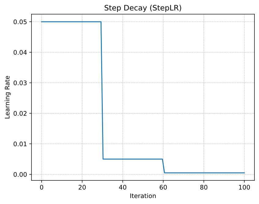
1. Step Decay

Reduce the learning rate by a factor (e.g., 0.1) every few epochs (e.g., every 10 epochs).

$\boxed{\eta_{t+1} = \gamma \eta_t \quad \text{every } k \text{ epochs}}$

Analogy: Step decay is like driving at high speed initially, then periodically reducing speed as you get closer to your destination.

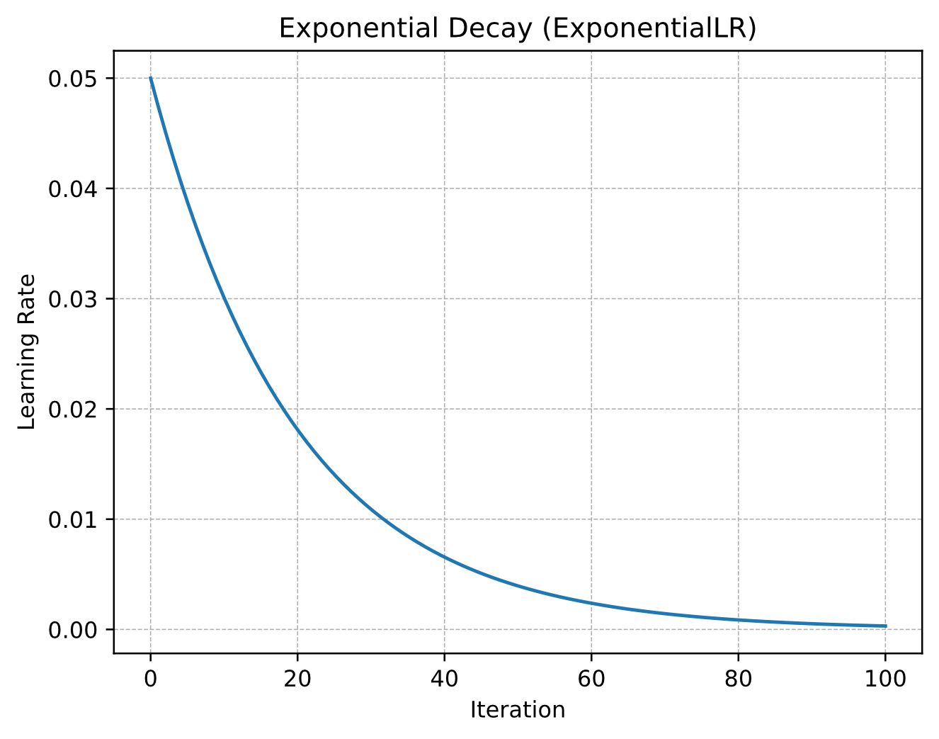
2. Exponential Decay

Decrease the learning rate exponentially over time, typically using a decay rate.

$\boxed{\eta_t = \eta_0 \cdot \gamma^t}$

Analogy: Exponential decay is like gradually and smoothly slowing down your car as you approach your destination, with the rate of slowing itself decreasing over time.

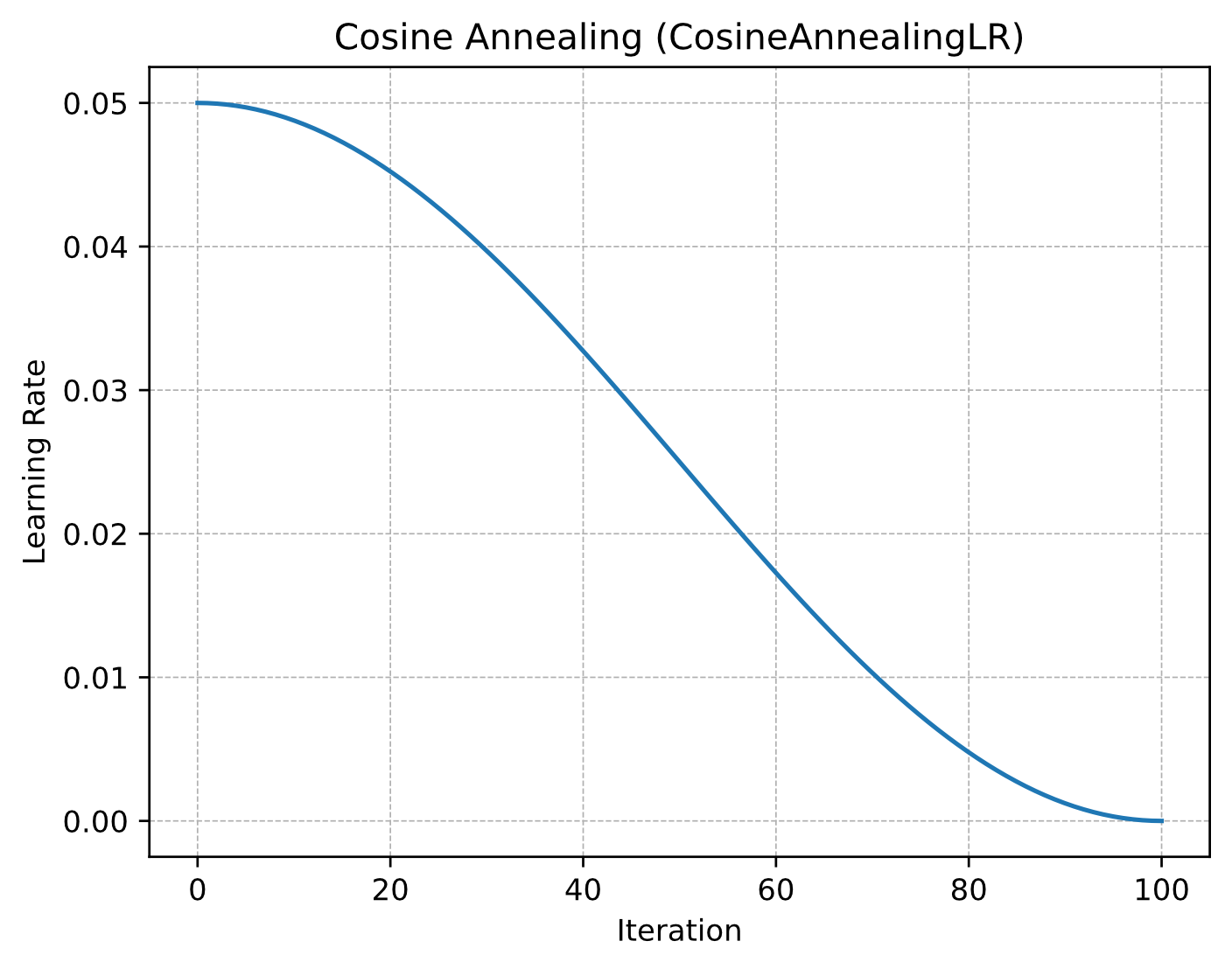
3. Cosine Annealing

Gradually decrease the learning rate following a cosine function.

$\boxed{\eta_t = \eta_{min} + \frac{1}{2}(\eta_{max} - \eta_{min})\left(1 + \cos\left(\frac{t\pi}{T}\right)\right)}$
where:

• $\eta_{min}$ and $\eta_{max} = \eta_0$ are the minimum and maximum learning rates
• $T$ is the total number of iterations

Analogy: Cosine annealing is like a smooth, wave-like deceleration. It starts fast, slows down smoothly in a curved pattern, and gently approaches the minimum, like a pendulum gradually coming to rest.

10.10 Summary

• Gradient Descent (GD) is an optimization algorithm used to minimize the loss function by iteratively updating model parameters in the direction of the negative gradient
• Stochastic Gradient Descent (SGD) is a variant of GD that updates model parameters using a single sample or a small batch of samples, making it more efficient for large datasets
• Adam is an advanced optimization algorithm that combines the benefits of AdaGrad and RMSProp, using adaptive learning rates for each parameter based on first and second moment estimates of the gradients
• Scheduling the learning rate during training can help improve convergence and performance, with common strategies including:
  • Step decay
  • Exponential decay
  • Cosine annealing