Optimization in One Dimension
- The problem: Given f:R→R, find x that minimizes f(x)
- Such x is called a minimizer and often denoted x∗
อย่างใน Airline scheduling, they can model how they assign their crew, which pilot take which flight, ต่าง ๆ สุดท้ายก็คือ Minimize cost → Maximize the profit
Local vs Global Optimization
Visual Representation
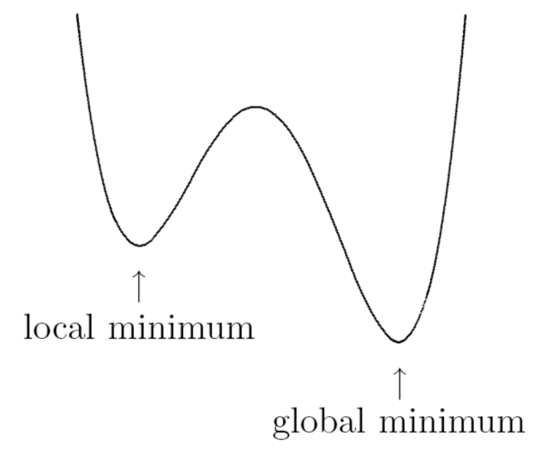
- Will cover only local optimization as global optimization is much more difficult to obtain
- (Informal) Definition: x∗ is a local minimizer of f when f(x∗) is smaller than or equal to the function values of all points near x∗
Analogy: Think of a local minimum like being in a valley in the mountains. You're at the lowest point in your immediate area (local), but there might be a deeper valley somewhere else on the mountain range (global). Global optimization is like finding the absolute lowest point across all valleys, which is much harder!
เหมือนว่าในบทนี้จะหาแค่ Local minimizer
คำถาม: ถ้าอยากหา Maximum บ้างล่ะ ซึ่งจริง ๆ แล้วมันคือสิ่งเดียวกัน แค่เปลี่ยนเครื่องหมายแล้วหา Minimum ซะ55555
Algorithm Steps
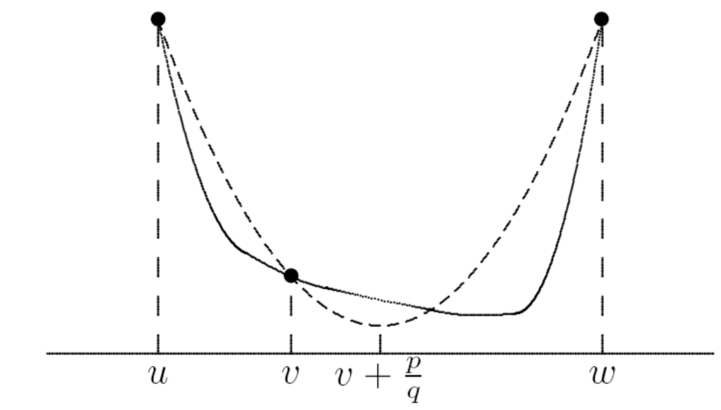
- Initially, evaluate f at three points
- Find the quadratic interpolant that fits the three points
- The minimum of the parabola interpolant (assuming it has one) is taken as a new approximate minimum of the function
Iteration Process
- At a given iteration, we have three points, say u, v, and w, with corresponding function values fu, fv, and fw, where v is the best approximate minimum of the function so far
- The minimum of the parabola interpolating the three points is given by:
v−21(v−u)(fv−fw)−(v−w)(fv−fu)(v−u)2(fv−fw)−(v−w)2(fv−fu)
- Replace u by w, w by v, and v by the new approximate minimum above (replace the oldest point, which is always u)
- Repeat until convergence
Visual Representation
Convergence Properties
- Successive parabolic interpolation is not guaranteed to converge
- But if started close enough to a minimum and the function is well-behaved, it converges superlinearly with convergence rate r≈1.324
Analogy: Imagine you're trying to find the bottom of a bowl by fitting curved slides (parabolas) through three points you've measured. Each time, you slide down to where your curved slide predicts the bottom is, then measure new points around there. If you start reasonably close to the actual bottom, you'll quickly zoom in on it!
Example 1: Successive Parabolic Interpolation
Problem: Minimize f(x)=0.5−xe−x2
Initial Setup
- Choose three initial points: x0=0, x1=1.2, and x2=0.6
- Evaluate:
- f(x0)=0.5−0e−02=0.5
- f(x1)=0.5−(1.2)e−(1.2)2=0.216
- f(x2)=0.5−(0.6)e−(0.6)2=0.081
Iteration Results
- The minimizer of the parabola fitting these three points by the formula is: x3=0.754
- แทนเข้าสูตรยาว ๆ เมื่อกี้ ได้ x3 ออกมา
- Discard x0 and repeat the process with the three remaining points x1, x2, and x3
Iteration Table
| k | xk | f(xk) |
|---|
| 0 | 0.000000 | 0.500000 |
| 1 | 1.200000 | 0.215687 |
| 2 | 0.600000 | 0.081394 |
| 3 | 0.754267 | 0.072981 |
| 4 | 0.720797 | 0.071278 |
| 5 | 0.708374 | 0.071119 |
| 6 | 0.706920 | 0.071118 |
| 7 | 0.707103 | 0.071118 |
Newton's Method for One-Dimensional Optimization
Derivation
-
The first three terms of Taylor series give:
f(x+h)≈f(x)+f′(x)h+21f′′(x)h2(1)
-
Suppose we know a point x(k) that is close to a minimizer of f
-
We want to find h such that f(x(k)+h) is minimized
-
Using the approximation in (1), let us instead find h such that
f(x(k))+f′(x(k))h+21f′′(x(k))h2=g(h)
is minimized
Finding the Minimum
- The minimum of g(h) (if exists) is the point where:
g′(h)=f′(x(k))+f′′(x(k))h=0
- Solve for h:
f'(x^{(k)}) + f''(x^{(k)})h &= 0 \\
f''(x^{(k)})h &= -f'(x^{(k)}) \\
h &= -\frac{f'(x^{(k)})}{f''(x^{(k)})}
\end{align}$$
- So $x^{(k)} + h = x^{(k)} - \left(f'(x^{(k)})/f''(x^{(k)})\right)$ is a new (hopefully better) approximation to the minimizer of $f$
- Repeat the iterative process
### Algorithm: Newton's Method for One-Dimensional Optimization
```
x^(0) = initial guess
for k = 0, 1, 2, ...
x^(k+1) = x^(k) - f'(x^(k))/f''(x^(k))
end
```
**Note**: Same as Newton's method for solving the nonlinear equation $f'(x) = 0$
**Convergence**: Therefore has **quadratic convergence** (under several assumptions)
> **Analogy**: Newton's method is like having a magic compass that points toward the minimum. At each step, you use both the slope (first derivative) and the curvature (second derivative) to figure out exactly how far to jump. If you're close enough to start, you'll converge extremely fast (errors square themselves each iteration)!
### Example 2: Newton's Method
**Problem**: Use Newton's method to minimize $f(x) = 0.5 - xe^{-x^2}$
#### Derivatives
- $f'(x) = (2x^2 - 1)e^{-x^2}$
- $f''(x) = 2x(3 - 2x^2)e^{-x^2}$
>ถ้า $f(x)$ มัน Complex มาก ๆ หา $f’(x)$ ไม่เป็น ก็สามารถใช้ [[9 - Numerical Differentiation#Finite Difference|Finite Difference]] to approximate the derivative
#### Newton Iteration Formula
$$x^{(k+1)} = x^{(k)} - \frac{f'(x^{(k)})}{f''(x^{(k)})}$$
$$x^{(k+1)} = x^{(k)} - \frac{(2(x^{(k)})^2 - 1)e^{-(x^{(k)})^2}}{2x^{(k)}(3 - 2(x^{(k)})^2)e^{-(x^{(k)})^2}}$$
$${x^{(k+1)} = x^{(k)} - \frac{2(x^{(k)})^2 - 1}{2x^{(k)}(3 - 2(x^{(k)})^2)}}$$
#### Results Starting from $x^{(0)} = 1$
| k | $x^{(k)}$ | $f(x^{(k)})$ |
| --- | --------- | ------------ |
| 0 | 1.000000 | 0.132121 |
| 1 | 0.500000 | 0.110600 |
| 2 | 0.700000 | 0.071162 |
| 3 | 0.707072 | 0.071118 |
| 4 | 0.707107 | 0.071118 |
![[CSS322_Doable_L12_Ex2.pdf]]
---
## Derivatives of Multivariate Functions
>ถ้า $f : \mathbb{R}^n \to \mathbb{R}^m$ ([[11 - Nonlinear Equations]]): First Derivative จะเรียกว่า Jacobian
>ถ้า $f : \mathbb{R}^n \to \mathbb{R}$ : First Derivative จะเรียกว่า Gradient
>ต่างกันนะ แม้ว่า Notation จะเหมือนกัน $\nabla f(x)$
### Gradient
- Suppose $f : \mathbb{R}^n \to \mathbb{R}$. The **gradient** of $f$ is the $n$-vector of partial derivatives:
$$\nabla f(x) = \begin{bmatrix} \frac{\partial f}{\partial x_1} \\
\frac{\partial f}{\partial x_2} \\
\vdots \\
\frac{\partial f}{\partial x_n}
\end{bmatrix}$$
where $x_i$ is the $i$-th entry of $x$
### Hessian Matrix
>มาเป็น Second derivative บ้างละ ทีนี้
- The **Hessian matrix** (second derivative) of $f : \mathbb{R}^n \to \mathbb{R}$ is the matrix:
$$\nabla^2 f(x) = \begin{bmatrix}
\frac{\partial^2 f}{\partial x_1^2} & \cdots & \frac{\partial^2 f}{\partial x_n \partial x_1} \\
\vdots & \ddots & \vdots \\
\frac{\partial^2 f}{\partial x_1 \partial x_n} & \cdots & \frac{\partial^2 f}{\partial x_n^2}
\end{bmatrix}$$
- That is: $\left[\nabla^2 f(x)\right]_{ij} = \frac{\partial^2 f}{\partial x_j \partial x_i} = \frac{\partial}{\partial x_j}\left(\frac{\partial f}{\partial x_i}\right)$
> [!NOTE] Theorem: Symmetry of Mixed Partials
> If both $\frac{\partial^2 f}{\partial x_j \partial x_i}$ and $\frac{\partial^2 f}{\partial x_i \partial x_j}$ are well-defined and continuous, then:
>$$\boxed{\frac{\partial^2 f}{\partial x_j \partial x_i} = \frac{\partial^2 f}{\partial x_i \partial x_j}}$$
> **Analogy**: The gradient is like a compass showing you which direction is uphill from where you're standing. The Hessian is like a topographic map showing how the terrain curves in all directions around you.
>For this course, ไม่ต้องห่วงว่าสองด้านจะไม่เท่ากัน จะเท่ากันหมด ไม่ยาก
### Example 3: Computing Gradient and Hessian
**Problem**: Find the gradient and the Hessian matrix of:
$$f(x) = x_1^2 + 3x_1x_2 + x_2^2 - x_1e^{x_2}$$
#### Solution
**Gradient**:
$$\nabla f(x) = \begin{bmatrix}
\frac{\partial f}{\partial x_1} \\
\frac{\partial f}{\partial x_2}
\end{bmatrix} = \begin{bmatrix}
2x_1 + 3x_2 - e^{x_2} \\
3x_1 + 2x_2 - x_1e^{x_2}
\end{bmatrix}$$
**Hessian**:
$$\nabla^2 f(x) = \begin{bmatrix}
\frac{\partial^2 f}{\partial x_1^2} & \frac{\partial^2 f}{\partial x_2 \partial x_1} \\
\frac{\partial^2 f}{\partial x_1 \partial x_2} & \frac{\partial^2 f}{\partial x_2^2}
\end{bmatrix} = \begin{bmatrix}
2 & 3 - e^{x_2} \\
3 - e^{x_2} & 2 - x_1e^{x_2}
\end{bmatrix}$$
- สังเกตว่าซ้ายล่าง - ขวาบน จะเท่ากัน ใช่เลยล่ะ
![[CSS322_Doable_L12_Ex3.pdf]]
___
## Unconstrained Optimization in Higher Dimensions
**Problem**: Given $f : \mathbb{R}^n \to \mathbb{R}$, find $x$ that minimizes $f(x)$
### Necessary and Sufficient Conditions for Local Minimizers
> [!NOTE] Theorem (Necessary Condition)
> - If $x^*$ is a local minimizer of $f$, then $\nabla f(x^*) = 0$ **and** $\nabla^2 f(x^*)$ is symmetric positive semidefinite
> - This is called the **necessary condition** of local minimizer
> [!NOTE] Theorem (Sufficient Condition):
>- If $x^*$ is a point such that $\nabla f(x^*) = 0$ **and** $\nabla^2 f(x^*)$ is symmetric positive definite, then $x^*$ is a local minimizer of $f$
>- This is called the **sufficient condition** of local minimizer
> **Analogy**: The necessary condition is like saying "if you're at the bottom of a valley, the ground must be flat (zero gradient) and curve upward in all directions (positive semidefinite Hessian)." The sufficient condition says "if you find such a point with definite upward curvature, you've definitely found a valley bottom!"
---
## Newton's Method for Multidimensional Optimization
### Taylor Series for Multivariate Functions
- Taylor series for $f : \mathbb{R}^n \to \mathbb{R}$ case (the first three terms):
$${f(x + h) \approx f(x) + (\nabla f(x))^T h + \frac{1}{2}h^T(\nabla^2
f(x))h}$$
>ถ้าเจอสัญลักษณ์ $\nabla f(x)$ ให้ note ด้วยว่ามันเป็น Jacobian หรือ Gradient
### Newton's Iteration Formula
Using similar derivation as in the one-dimension case, we have the iterates:
$$\boxed{x^{(k+1)} = x^{(k)} - \left(\nabla^2 f(x^{(k)})\right)^{-1} \nabla f(x^{(k)})}$$
**Important**: Remember to solve the linear system for $h^{(k)} = -\left(\nabla^2 f(x^{(k)})\right)^{-1} \nabla f(x^{(k)})$ rather than explicitly form the inverse
### Algorithm: Newton's Method for Unconstrained Optimization
```
x^(0) = initial guess
for k = 0, 1, 2, ...
Solve ∇²f(x^(k)) h^(k) = -∇f(x^(k)) for h^(k)
x^(k+1) = x^(k) + h^(k)
end
```
### Example 4: Newton's Method in 2D
**Problem**: Use Newton's method to minimize
$$f(x) = 0.5x_1^2 + 2.5x_2^2$$
starting with $x^{(0)} = \begin{bmatrix} 5 \\ 1 \end{bmatrix}$
#### Solution
The derivatives are:
$$\nabla f(x) = \begin{bmatrix} x_1 \\ 5x_2 \end{bmatrix}, \quad \nabla^2 f(x) = \begin{bmatrix} 1 & 0 \\ 0 & 5 \end{bmatrix}$$
At $x^{(0)} = \begin{bmatrix} 5 \\ 1 \end{bmatrix}$:
$$\nabla f(x^{(0)}) = \begin{bmatrix} 5 \\ 5 \end{bmatrix}$$
The linear system to solve is:
$$\begin{bmatrix} 1 & 0 \\ 0 & 5 \end{bmatrix} h^{(0)} = \begin{bmatrix} -5 \\ -5 \end{bmatrix}$$
The solution is:
$$h^{(0)} = \begin{bmatrix} -5 \\ -1 \end{bmatrix}$$
Therefore:
$$x^{(1)} = x^{(0)} + h^{(0)} = \begin{bmatrix} 5 \\ 1 \end{bmatrix} + \begin{bmatrix} -5 \\ -1 \end{bmatrix} = \begin{bmatrix} 0 \\ 0 \end{bmatrix}$$
which is the exact solution for this problem!
**Note**: Because $f$ in this example is quadratic, Newton's method converges in one iteration. This is not true in general, however.
![[Screenshot 2025-10-26 at 2.16.05 PM.png|center|400]]
![[CSS322_Doable_L12_Ex4.pdf]]
### Comments on Newton's Method for Optimization
- Just like in the nonlinear case, Newton's method for unconstrained optimization converges **quadratically** if started close enough to a solution
- Otherwise, it may not converge or converge more slowly
#### Properties When $f$ has Continuous Second Partial Derivatives
- The Hessian matrix is **symmetric**
- Near a minimum, it is **positive definite** ⇒ So use [[6 - More on Solving Linear Systems#Cholesky Factorization|Cholesky factorization]] to solve the linear system for $h^{(k)}$
- If far from a minimum, the Hessian is symmetric but not positive definite
- There are algorithms for solving a linear system with such matrices
---
## Secant Updating Methods
### Motivation
- Just like in the nonlinear case, we may not want to compute the true Hessian matrix each iteration as it is **expensive**
- **One approach**: Use [[11 - Nonlinear Equations#4. Broyden's Method|Broyden's method]] to find a zero of the gradient
- **Disadvantage**: This approach cannot preserve the symmetry of the Hessian matrix
### BFGS Method
- Many secant updating methods for optimization exist
- One of the most effective is the **BFGS method**
- Similar to [[11 - Nonlinear Equations#4. Broyden's Method|Broyden's method]], BFGS updates the approximation of the Hessian matrix each iteration
> **Analogy**: Computing the exact Hessian every iteration is like recalculating your entire GPS route from scratch at every step. Secant methods like BFGS are like making smart adjustments to your route based on where you've been, which is much faster while still getting you to your destination!
## BFGS Algorithm
>Method ใหม่เลย idea จาก [[#Newton's Iteration Formula]]
>อันนี้ออกสอบมั้ย? ถามอาจารย์
### Algorithm: BFGS Method for Unconstrained Optimization
```
x^(0) = initial guess
B^(0) = initial Hessian approximation
For k = 0, 1, 2, ...
Solve B^(k) h^(k) = -∇f(x^(k)) for h^(k)
x^(k+1) = x^(k) + h^(k)
y^(k) = ∇f(x^(k+1)) - ∇f(x^(k))
B^(k+1) = B^(k) + (y^(k)(y^(k))^T) / ((y^(k))^T h^(k))
- (B^(k) h^(k) (h^(k))^T B^(k)) / ((h^(k))^T B^(k) h^(k))
Endfor
```
### Key Properties of BFGS
- The initial $B^{(0)}$ can be set to $I$ or the true or approximated Hessian
- In practice, a **factorization** of $B^{(k)}$ is updated rather than $B^{(k)}$ itself
- This reduces the cost per iteration from $O(n^3)$ to $O(n^2)$ operations
- BFGS normally has a **superlinear convergence rate** although the approximate Hessian may not converge to the true Hessian
---
## Summary
### One-Dimensional Optimization Methods
1. **Successive Parabolic Interpolation**
- Fit parabolas through 3 points
- Convergence rate: $r \approx 1.324$ (superlinear)
- Not guaranteed to converge
2. **Newton's Method**
- Uses first and second derivatives
- Convergence: Quadratic (when close to solution)
- Formula: $\boxed{x^{(k+1)} = x^{(k)} - \frac{f'(x^{(k)})}{f''(x^{(k)})}}$
### Multidimensional Optimization Methods
1. **Newton's Method**
- Solve: $\nabla^2 f(x^{(k)}) h^{(k)} = -\nabla f(x^{(k)})$
- Update: $x^{(k+1)} = x^{(k)} + h^{(k)}$
- Convergence: Quadratic (near solution)
2. **BFGS Method**
- Approximates Hessian using secant updates
- Cost: $O(n^2)$ per iteration (vs $O(n^3)$ for Newton)
- Convergence: Superlinear
### Key Conditions for Local Minimizers
- **Necessary**: $\nabla f(x^*) = 0$ and $\nabla^2 f(x^*)$ is positive semidefinite
- **Sufficient**: $\nabla f(x^*) = 0$ and $\nabla^2 f(x^*)$ is positive definite