บาง method ให้จุด บาง method v (function ที่ simpler)
โจทย์ให้มา:
ให้สมการอนุพันธ์อันดับสอง เช่น
u′′=f(t,u,u′)
และให้ค่าที่ “ปลายทั้งสองข้าง” เช่น
u(a)=α, u(b)=β
เราต้องการหา:
ฟังก์ชัน u(t) ที่ทำให้ตรงตามเงื่อนไข ทั้งสองปลาย
Overview
- We focus on second-order scalar boundary value problems (BVPs)
- BVPs are given by second-order scalar ODEs:
u′′=f(t,u,u′),a<t<b
- With boundary conditions:
u(a)=α,u(b)=β
where α and β are given scalar constants.
Physical Applications
Many important physical problems have this form:
- Elastic beam bending under a distributed load
- Electrical potential distribution between two flat electrodes
- Temperature distribution in an internally heated homogeneous wall whose surfaces are maintained at fixed temperature
- Steady-state concentration of a pollutant in porous soil
Analogy: Think of a BVP like a tightrope walk where you know where the rope is attached at both ends (boundary conditions), but you need to figure out the shape of the rope in between. Unlike initial value problems (IVPs) where you start at one point and march forward, BVPs require you to satisfy conditions at both ends simultaneously.
Existence and Uniqueness of Solutions
สำหรับ Boundary Value Problem (BVP) บางครั้ง “อาจไม่มีคำตอบเลย” หรือ “อาจมีหลายคำตอบก็ได้” ไม่เหมือน IVP ที่ส่วนใหญ่มีคำตอบเดียวแน่นอน
Key Concept
- Solutions to BVPs may not exist
- If they do exist, they may not be unique
Example: Non-Unique Solutions
Consider the BVP:
u′′=−u,0<t<b
with boundary conditions:
u(0)=0,u(b)=β
where b is an integer multiple of π.
Analysis:
- The general solution of the ODE satisfying u(0)=0 is u(t)=csin(t) for any constant c
- Because b is an integer multiple of π: csin(b)=0 for any c
- Result:
- Infinitely many solutions if β=0
- No solution if β=0
Analogy: Imagine trying to connect two dots with a sine wave. If the second dot happens to land exactly where the sine wave naturally crosses zero, you have infinite ways to do it (any amplitude works). But if the second dot is anywhere else, it's impossible to hit it with a sine wave starting from zero.
Method 1: Shooting Method
Method for solving second-order BVPs
Main Idea
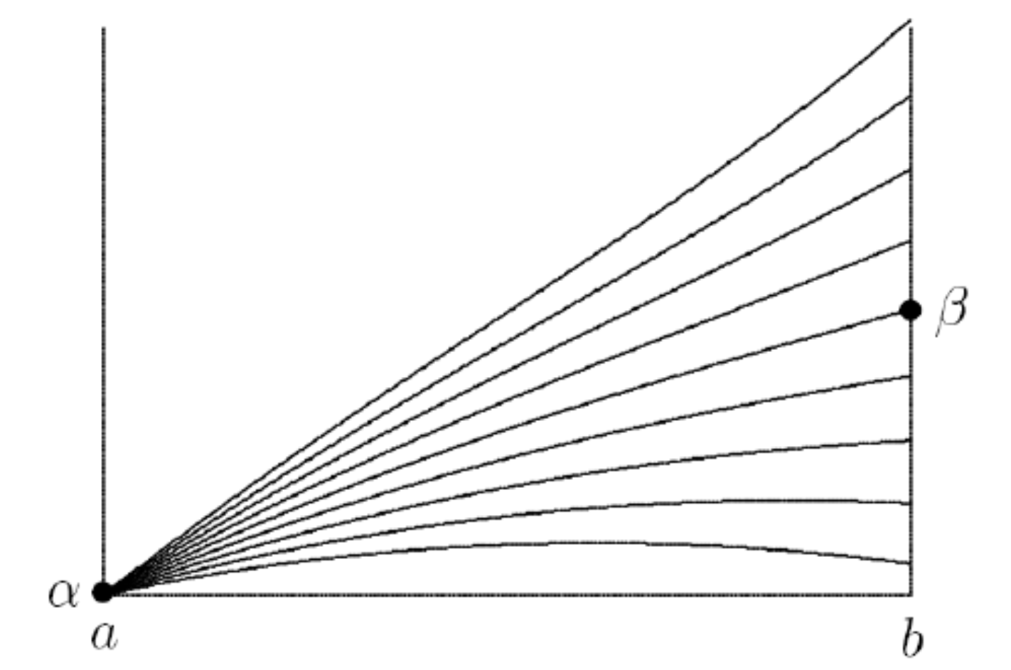
The shooting method approximately satisfies the ODE from the start and iterates until the boundary conditions are satisfied.
Setup
Recall the problem:
u′′=f(t,u,u′),a<t<b
u(a)=α,u(b)=β
Convert to first-order system:
13 - Initial Value Problems for Ordinary Differential Equations (IVP)
[y1′y2′]=[y2f(t,y1,y2)],a<t<b
where:
- y1(t)=u(t)
- y2(t)=u′(t)
Key observation:
- We know y1(a)=u(a)=α
- Note: If we also knew y2(a)=u′(a), then we would have an IVP!
Algorithm
Step 1: Guess u′(a)
Step 2: Solve the resulting IVP
Step 3: Check if the computed solution value at t=b is equal to β (the desired boundary value)
Step 4: If yes, the computed solution is the correct one for the BVP
Step 5: Otherwise, try different u′(a) and repeat (using the previous results for the new guess u′(a))
Analogy: The shooting method is like adjusting the angle of a cannon to hit a target. You know where you're starting (the cannon's position) and where you want to end up (the target), but you don't know the initial angle. You fire, see where you land, adjust the angle based on whether you overshot or undershot, and try again.
Visual Representation
Image on page 6 showing multiple trajectory curves from point α at a trying to hit point β at b
Example 1: Shooting Method
Consider using the shooting method on:
u′′=6t,0<t<1
with boundary conditions:
u(0)=0,u(1)=1
Transform to first-order system:
[y1′y2′]=[y26t]
where y1(t)=u(t) and y2(t)=u′(t).
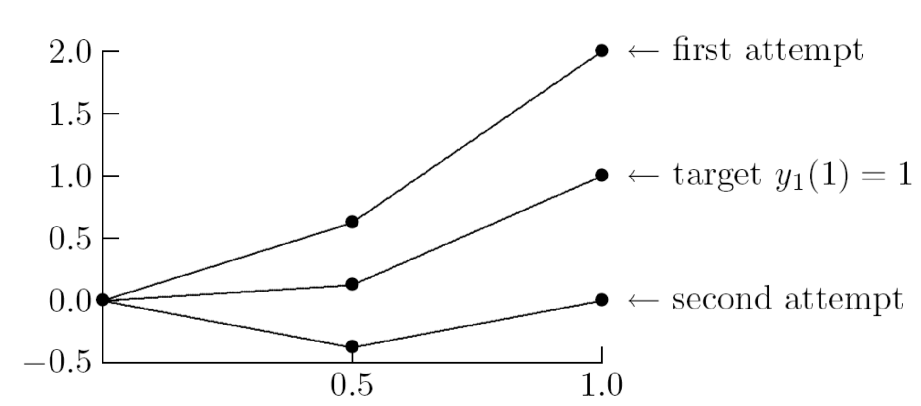
Attempt 1: Try y2(0)=1
Using fourth-order Runge-Kutta method with step size h=0.5:
- At t1=0.5: y1=[0.6251.750]
- At t2=1: y2=[2.04.0]
- Result: We hit y1(1)=2 instead of the desired value y1(1)=1 ❌
Attempt 2: Try y2(0)=−1
With these new initial values:
-
At t1=0.5:
y1=[−0.375−0.250]
-
At t2=1:
y2=[0.02.0]
-
Result: We hit y1(1)=0 instead of the desired value y1(1)=1 ❌
-
Conclusion: The correct initial slope is somewhere between −1 and 1
Attempt 3: Try y2(0)=0 ✓
Eventually we get to the correct initial slope y2(0)=0:
y2=[1.03.0]
- Success! This hits the target boundary value y1(1)=1 ✓
Drawbacks of Shooting Method
Problem 1: The associated IVP may be unstable even when the BVP is stable
Problem 2: For some starting guesses, the solution of the IVP may become unbounded before reaching the right-hand endpoint of the BVP
Analogy: Sometimes the cannon analogy breaks down because the cannonball might explode mid-flight (instability) or fly off to infinity instead of landing anywhere useful. This is especially problematic for stiff equations or long intervals.
Method 2: Finite Difference Method
Main Idea
Key Question: How about satisfying the boundary conditions from the start and iterating until the ODE is approximately satisfied?
Setup
Given:
u′′=f(t,u,u′),a<t<b
u(a)=α,u(b)=β
Discretization:
- Introduce mesh points: ti=a+ih, for i=0,…,n+1
- Where h=n+1b−a
- We want approximate solution values: yi≈u(ti) for i=1,…,n
- We already have: y0=u(a)=α and yn+1=u(b)=β
Finite Difference Approximations
Replace derivatives with finite difference approximations:
u′(ti)≈2hyi+1−yi−1
u′′(ti)≈h2yi+1−2yi+yi−1
Important: Choose formulas with the same order of accuracy (the accuracy is limited by the least accurate formula)
Resulting System
Substituting into the ODE:
h2yi+1−2yi+yi−1=f(ti,yi,2hyi+1−yi−1)
- This is a system of n equations in n unknowns: y1,y2,…,yn
- The system may be linear or nonlinear depending on f
- If nonlinear, use values on a straight line between (a,α) and (b,β) as starting guesses for the iterative method
Analogy: Instead of shooting from one end, we're laying out a grid of points and trying to satisfy the differential equation at each grid point, like placing fence posts at regular intervals and making sure the fence satisfies certain height requirements at each post.
Example 2: Finite Difference Method ex2.py
ได้ออกมาเป็นจุด
Let's try the finite difference method on the same BVP:
u′′=6t,0<t<1
u(0)=0,u(1)=1
Setup:
- Use one interior mesh point: t1=0.5
- Total of three mesh points (including boundaries): t0=0,t1=0.5,t2=1
- From boundary conditions: y0=u(t0)=0 and y2=u(t2)=1
Finite difference at t1:
h2y2−2y1+y0=f(t1,y1,2hy2−y0)
Substitute values:
(0.5)21−2y1+0=6(0.5)
0.251−2y1=3
4−8y1=3
u(0.5)≈y1=81=0.125
Example 3: More Complex Finite Difference
Consider the BVP:
u′′=t2u+tu′,2<t<4
u(2)=2,u(4)=−1
Using three interior mesh points (n=3).
Setup:
- h=n+1b−a=3+14−2=0.5
- Mesh points: t0=2,t1=2.5,t2=3,t3=3.5,t4=4
- Boundary conditions: y0=2,y4=−1
Finite difference equations (for i=1,2,3):
h2yi+1−2yi+yi−1=ti2yi+ti(2hyi+1−yi−1)
Using Centered Differences for Both Derivatives
9 - Numerical Differentiation
The system of equations becomes:
(0.5)2y2−2y1+y0=(2.5)2y1+(2.5)(2(0.5)y2−y0)
(0.5)2y3−2y2+y1=32y2+3(2(0.5)y3−y1)
(0.5)2y4−2y3+y2=(3.5)2y3+(3.5)(2(0.5)y4−y2)
Substitute y0=2 and y4=−1, then simplify:
-14.25y_1 + 1.5y_2 &= 13 \\
7y_1 - 17y_2 + y_3 &= 0 \\
7.5y_2 - 20.25y_3 &= 0.5
\end{aligned}}$$
This linear system can be solved for $y_1, y_2, y_3$.
#### Alternative: Backward Difference for $u'$
**Not recommended in practice**, but for illustration:
Using backward difference for $u'$ and centered difference for $u''$:
$$\frac{y_{i+1} - 2y_i + y_{i-1}}{h^2} = t_i^2 y_i + t_i\left(\frac{y_i - y_{i-1}}{h}\right)$$
The system becomes:
$$\frac{y_2 - 2y_1 + y_0}{(0.5)^2} = (2.5)^2y_1 + (2.5)\left(\frac{y_1 - y_0}{0.5}\right)$$
$$\frac{y_3 - 2y_2 + y_1}{(0.5)^2} = 3^2y_2 + 3\left(\frac{y_2 - y_1}{0.5}\right)$$
$$\frac{y_4 - 2y_3 + y_2}{(0.5)^2} = (3.5)^2y_3 + (3.5)\left(\frac{y_3 - y_2}{0.5}\right)$$
Then substitute $y_0 = 2$ and $y_4 = -1$ and solve.
> **Note**: Using different order approximations (e.g., $O(h)$ backward difference with $O(h^2)$ centered difference) reduces overall accuracy to the lower order. Always match the orders!
---
## Method 3: Collocation Method
### Main Idea
- Approximate the solution $u(t)$ by a function $v(t, x)$ whose derivatives can be computed **analytically**
- Make sure that $v(t, x)$ satisfies the ODE at a number of points (collocation points)
>Method ก่อนหน้านี้จะให้ A number of discrete point approximate $u(t)$ แต่อันนี้เราจะได้ simpler function $v$ approximate $u$ ???
### Setup
Given:
$$u'' = f(t, u, u'), \quad a < t < b$$
$$u(a) = \alpha, \quad u(b) = \beta$$
**Approximate solution form:**
$$\boxed{u(t) \approx v(t, x) = \sum_{i=1}^{n} x_i \phi_i(t)}$$
where:
- $\phi_i(t)$ are **basis functions** whose derivatives can be computed analytically
- Examples: polynomials, trigonometric functions
- $x_i$ are the **coefficients** we want to find
### Collocation Process
**Define** $n$ collocation points: $a = t_1 < \cdots < t_n = b$
**Force** $v(t, x)$ to:
1. **Satisfy the ODE** at interior collocation points:
$$v''(t_i, x) = f(t_i, v(t_i, x), v'(t_i, x)), \quad i = 2, \ldots, n-1$$
2. **Satisfy the boundary conditions** at endpoints:
$$v(t_1, x) = \alpha, \quad v(t_n, x) = \beta$$
**Key advantage:** $v''$ and $v'$ can be computed exactly analytically!
**Result:** A system of $n$ equations in $n$ unknowns that we can solve for $x$
> **Analogy**: Collocation is like fitting a smooth curve (made from basis functions) through a set of posts (collocation points), where the curve must satisfy both the differential equation rules and the boundary fence heights. It's more flexible than finite differences because you can choose sophisticated basis functions that naturally satisfy certain properties.
### Example 4: Collocation with Polynomials
Consider the BVP:
$$u'' = 6t, \quad 0 < t < 1$$
$$u(0) = 0, \quad u(1) = 1$$
**Setup:**
- Use one interior collocation point: $t_2 = 0.5$
- Total collocation points: $t_1 = 0, t_2 = 0.5, t_3 = 1$
- Use **monomial basis**: $v(t, x) = x_1 + x_2t + x_3t^2$ ([[7 - Interpolation]]) (โจทย์ให้)
**Derivatives:**
$$v'(t, x) = x_2 + 2x_3t$$$$v''(t, x) = 2x_3$$
#### Satisfy ODE at $t_2 = 0.5$
$$v''(t_2, x) = f(t_2, v(t_2, x), v'(t_2, x))$$
$$2x_3 = 6t_2$$
$$2x_3 = 6(0.5) = 3$$
$$\boxed{x_3 = 1.5}$$
#### Satisfy Left Boundary Condition
$$v(t_1, x) = 0$$
$$x_1 + x_2t_1 + x_3t_1^2 = 0$$
$$x_1 + x_2(0) + x_3(0) = 0$$
$$\boxed{x_1 = 0}$$
#### Satisfy Right Boundary Condition
$$v(t_3, x) = 1$$
$$x_1 + x_2t_3 + x_3t_3^2 = 1$$
$$x_1 + x_2 + x_3 = 1$$
$$0 + x_2 + 1.5 = 1$$
$$\boxed{x_2 = -0.5}$$
**Final approximate solution:**
$$\boxed{u(t) \approx -0.5t + 1.5t^2}$$
### Example 5: Collocation with Trigonometric Functions
Consider the BVP:
$$u'' = t^2u + tu', \quad 2 < t < 4$$
$$u(2) = 2, \quad u(4) = -1$$
**Setup:**
- One interior collocation point: $t_2 = 3$
- Total points: $t_1 = 2, t_2 = 3, t_3 = 4$
- Use **trigonometric basis**: $v(t, x) = x_1\cos t + x_2\sin t + x_3\cos(2t)$
**Derivatives:**
$$v'(t, x) = -x_1\sin t + x_2\cos t - 2x_3\sin(2t)$$
$$v''(t, x) = -x_1\cos t - x_2\sin t - 4x_3\cos(2t)$$
#### Satisfy ODE at $t_2 = 3$
$$v''(t_2, x) = t_2^2 v(t_2, x) + t_2v'(t_2, x)$$
$$\begin{aligned}
&-x_1\cos(3) - x_2\sin(3) - 4x_3\cos(6) = \\
&\quad (3)^2(x_1\cos(3) + x_2\sin(3) + x_3\cos(6)) \\
&\quad + 3(-x_1\sin(3) + x_2\cos(3) - 2x_3\sin(6))
\end{aligned}$$
#### Satisfy Left Boundary Condition
$$v(2, x) = 2$$
$$x_1\cos(2) + x_2\sin(2) + x_3\cos(4) = 2$$
#### Satisfy Right Boundary Condition
$$v(4, x) = -1$$
$$x_1\cos(4) + x_2\sin(4) + x_3\cos(8) = -1$$
**Solve** the system of three equations for $x_1, x_2, x_3$ to obtain $v(t, x)$.
### Example 6: Nonlinear Collocation
Consider the BVP:
$$u'' = \frac{u^2}{u'}, \quad 1 < t < 3$$
$$u(1) = -1, \quad u(3) = 1$$
**Setup:**
- Two interior collocation points: $t_2 = 1.5, t_3 = 2$
- Total points: $t_1 = 1, t_2 = 1.5, t_3 = 2, t_4 = 3$
- Use **polynomial basis**: $v(t, x) = x_1 + x_2t + x_3t^2 + x_4t^3$
**Derivatives:**
$$v'(t, x) = x_2 + 2x_3t + 3x_4t^2$$
$$v''(t, x) = 2x_3 + 6x_4t$$
#### Satisfy ODE at $t_2 = 1.5$
$$v''(t_2, x) = \frac{v(t_2, x)^2}{v'(t_2, x)}$$
$$2x_3 + 6x_4(1.5) = \frac{\left(x_1 + x_2(1.5) + x_3(1.5)^2 + x_4(1.5)^3\right)^2}{x_2 + 2x_3(1.5) + 3x_4(1.5)^2}$$
#### Satisfy ODE at $t_3 = 2$
$$v''(t_3, x) = \frac{v(t_3, x)^2}{v'(t_3, x)}$$
$$2x_3 + 6x_4(2) = \frac{\left(x_1 + x_2(2) + x_3(2)^2 + x_4(2)^3\right)^2}{x_2 + 2x_3(2) + 3x_4(2)^2}$$
#### Satisfy Boundary Conditions
Left boundary:
$$v(1, x) = -1$$
$$x_1 + x_2 + x_3 + x_4 = -1$$
Right boundary:
$$v(3, x) = 1$$
$$x_1 + 3x_2 + 9x_3 + 27x_4 = 1$$
**Solve** the **nonlinear system** of 4 equations for $x_1, x_2, x_3, x_4$ to obtain $v(t, x)$.
### Comments about Collocation Method
**Important Note:**
- Satisfying the ODE at collocation points does **NOT** mean the approximate solution is exact at these points in general
- In general: $v(t_i, x) \neq u(t_i)$ for $i = 2, \ldots, n-1$
**Convergence:**
- Increasing the number of collocation points should cause the approximate solution to converge to the true solution
- Subject to the stability of the method and other factors
---
### Types of Collocation Methods
**Spectral Methods** (or **Pseudospectral Methods**)
- Use basis functions that are **nonzero almost over the entire problem domain**
- Examples: Fourier series, Chebyshev polynomials
- Excellent for smooth solutions
- Global approximation
**Finite Element Methods**
- Use basis functions that are **nonzero on only a small portion of the problem domain**
- Examples: piecewise linear functions, B-splines
- Better for non-smooth solutions or complex geometries
- Local approximation
> **Analogy**: Spectral methods are like describing a mountain range using a combination of smooth, global waves (sine and cosine functions) - great for smooth landscapes. Finite element methods are like connecting many small, simple pieces (like triangular facets) - better for rough terrain with sharp features.
---
## Summary Comparison of Methods
| Method | Key Idea | Advantages | Disadvantages |
|--------|----------|------------|---------------|
| **Shooting** | Guess initial derivative, solve IVP | - Uses existing IVP solvers<br>- Intuitive | - May be unstable<br>- Solutions may blow up<br>- Requires root-finding |
| **Finite Difference** | Discretize domain, approximate derivatives | - Straightforward<br>- Works for general problems | - Limited accuracy<br>- Large systems for high accuracy |
| **Collocation** | Fit smooth function through points | - Can achieve high accuracy<br>- Flexible choice of basis | - Requires solving system<br>- Basis function selection matters |
---
## Key Takeaways
✓ **BVPs are fundamentally different from IVPs**
- Conditions specified at boundaries, not just initial point
- Solutions may not exist or be unique
✓ **Shooting Method**: Convert BVP to IVP by guessing missing initial conditions
- Like aiming a cannon to hit a target
✓ **Finite Difference Method**: Satisfy boundaries exactly, approximate ODE on grid
- Like placing fence posts at regular intervals
✓ **Collocation Method**: Use smooth basis functions, satisfy ODE at specific points
- Like fitting a smooth curve through control points
✓ **Method selection depends on**:
- Problem characteristics (smoothness, domain, nonlinearity)
- Desired accuracy
- Available computational resources
- Stability requirements
---
## Mathematical Formulas Reference
### Finite Difference Formulas
**First derivative (centered):**
$$u'(t_i) \approx \frac{y_{i+1} - y_{i-1}}{2h} \quad \text{(2nd order)}$$
**Second derivative (centered):**
$$u''(t_i) \approx \frac{y_{i+1} - 2y_i + y_{i-1}}{h^2} \quad \text{(2nd order)}$$
**First derivative (backward):**
$$u'(t_i) \approx \frac{y_i - y_{i-1}}{h} \quad \text{(1st order)}$$
### Standard BVP Form
$$\boxed{u'' = f(t, u, u'), \quad a < t < b}$$
$$\boxed{u(a) = \alpha, \quad u(b) = \beta}$$
### Mesh Setup
$$t_i = a + ih, \quad h = \frac{b-a}{n+1}, \quad i = 0, 1, \ldots, n+1$$
# Method 4: Residual Methods
>ได้เป็น Function
## Introduction to Residual Methods
### Problem Setup
- Consider the scalar **Poisson equation** in one dimension:
$$u'' = f(t), \quad a < t < b$$
- With **homogeneous boundary conditions**:
$$u(a) = 0, \quad u(b) = 0$$
> **Note**: "Homogeneous" means the boundary values are both zero. This is like having a rope tied down at both ends at ground level.
### Approximate Solution Form
- Just like in collocation methods, find an approximate solution as a linear combination of basis functions:
$$\boxed{u(t) \approx v(t, x) = \sum_{i=1}^{n} x_i \phi_i(t)}$$
where:
- $\phi_i(t)$ are basis functions
- $x_i$ are coefficients to be determined
## The Residual Concept
### Definition of Residual
- Substituting $v(t, x)$ into the ODE:
$$v''(t, x) = f(t)$$
- Since the true solution $u(t)$ is **unlikely to be a linear combination** of the chosen basis functions, we consider minimizing the **residual**:
$$\boxed{r(t, x) = v''(t, x) - f(t) = \sum_{i=1}^{n} x_i \phi_i''(t) - f(t)}$$
> **Analogy**: The residual is like the "error" or "mismatch" between what our approximate solution gives us and what the differential equation actually requires. We want to make this error as small as possible.
### Partial Derivative of Residual
- For $i = 1, \ldots, n$:
$$\frac{\partial r}{\partial x_i} = \phi_i''(t)$$
## Method 1: Least-Squares Method
>There are many ways to minimize the residual อีก ก็ดูกันละกันมีกี่อัน
### Main Idea
- The **least-squares method** minimizes the squared residual integrated over the domain:
$$\boxed{F(x) = \frac{1}{2} \int_a^b r(t, x)^2 \, dt}$$
> **Analogy**: This is like finding the curve that has the smallest total squared error across the entire interval. Think of minimizing the total area between your approximate curve and the perfect solution.
>สมการด้านบนเหมือน Linear Least Square เลยแต่แค่ r เป็น continuous function
### Deriving the System
- The gradient of $F$ at the minimizer is zero
- For $i = 1, \ldots, n$:
$$0 = \frac{\partial F}{\partial x_i} = \int_a^b r(t, x) \frac{\partial r}{\partial x_i} \, dt = \int_a^b r(t, x) \phi_i''(t) \, dt$$
### Expanding the Equation
$$\begin{aligned}
0 &= \int_a^b r(t, x) \phi_i''(t) \, dt \\
&= \int_a^b \left( \sum_{j=1}^{n} x_j \phi_j''(t) - f(t) \right) \phi_i''(t) \, dt \\
&= \sum_{j=1}^{n} \left( \int_a^b \phi_j''(t) \phi_i''(t) \, dt \right) x_j - \int_a^b f(t) \phi_i''(t) \, dt
\end{aligned}$$
### Linear System Form
- This gives us:
$$\boxed{\sum_{j=1}^{n} \left( \int_a^b \phi_j''(t) \phi_i''(t) \, dt \right) x_j = \int_a^b f(t) \phi_i''(t) \, dt}$$
for $i = 1, \ldots, n$
- This is a **symmetric system** of linear equations $Ax = b$ where:
$$\boxed{a_{ij} = \int_a^b \phi_j''(t) \phi_i''(t) \, dt}$$
$$\boxed{b_i = \int_a^b f(t) \phi_i''(t) \, dt}$$
### Computing the System
- To obtain $A$ and $b$, we can either:
- Integrate **analytically** (exact formulas)
- Integrate **numerically** (using quadrature methods)
- Solving this system gives us $x$, which defines the approximate solution $v(t, x)$
## Example 7: Least-Squares Method
### Problem Statement
Try the least-squares method on the Poisson BVP:
$$u'' = e^t, \quad 3 < t < 7$$
with homogeneous boundary conditions:
$$u(3) = 0, \quad u(7) = 0$$
### Approximate Solution
- Approximate the solution $u$ with:
$$v(t, x) = x_1 \cos t + x_2 \sin t$$
- That is:
- $\phi_1(t) = \cos t$
- $\phi_2(t) = \sin t$
### Derivatives
$$\phi_1'(t) = -\sin t, \quad \phi_2'(t) = \cos t$$
$$\phi_1''(t) = -\cos t, \quad \phi_2''(t) = -\sin t$$
### Setting Up the System
- We solve the symmetric $2 \times 2$ system $Ax = b$ where:
$$a_{ij} = \int_a^b \phi_j''(t) \phi_i''(t) \, dt$$
$$b_i = \int_a^b f(t) \phi_i''(t) \, dt$$
### Computing the Right-Hand Side Vector $b$
$$\begin{aligned}
b_1 &= \int_a^b f(t) \phi_1''(t) \, dt = \int_3^7 e^t(-\cos t) \, dt = -\int_3^7 e^t(\cos t) \, dt \\
b_2 &= \int_a^b f(t) \phi_2''(t) \, dt = \int_3^7 e^t(-\sin t) \, dt = -\int_3^7 e^t(\sin t) \, dt
\end{aligned}$$
### Computing the Matrix $A$
$$\begin{aligned}
a_{11} &= \int_a^b \phi_1''(t) \phi_1''(t) \, dt = \int_3^7 (-\cos t)(-\cos t) \, dt = \int_3^7 (\cos^2 t) \, dt \\
\\
a_{12} &= \int_a^b \phi_2''(t) \phi_1''(t) \, dt = \int_3^7 (-\sin t)(-\cos t) \, dt = \int_3^7 \sin t \cos t \, dt \\
\\
a_{21} &= \int_a^b \phi_1''(t) \phi_2''(t) \, dt = \int_3^7 (-\cos t)(-\sin t) \, dt = \int_3^7 \sin t \cos t \, dt \\
\\
a_{22} &= \int_a^b \phi_2''(t) \phi_2''(t) \, dt = \int_3^7 (-\sin t)(-\sin t) \, dt = \int_3^7 (\sin^2 t) \, dt
\end{aligned}$$
- จะ Solve Integral ด้านขวามือก็ไม่ได้ยากขนาดนั้น อาจจะมีบอกว่าได้อะไรเลยใน some table, หรือว่าใช้ [[8 - Numerical Integration#n-point Quadrature|Quadrature rules]]
### Final Step
- Solve the system $Ax = b$ for $x$ to obtain the approximate solution $v(t, x)$
---
## Method 2: Weighted Residual Methods
### General Concept
- More general than minimizing $F(x)$
- A **weighted residual method** forces the residual to be **orthogonal** to each of a given set of **weight functions** (or **test functions**) $w_i$
- For $i = 1, \ldots, n$:
$$\boxed{\int_a^b r(t, x) w_i(t) \, dt = 0} \quad \text{(1)}$$
> **Analogy**: Instead of minimizing the overall error, we're saying "the error must be perpendicular to certain test directions." It's like requiring the error to have zero component in specific directions we care about.
### Connection to Least-Squares
- **Note**: The least-squares method is of this type with $w_i(t) = \phi_i''(t)$
- The **accuracy** of such methods depends on the choice of the weight functions
### Linear System
- Similar to before, equation (1) yields a linear system $Ax = b$ where:
$$\boxed{a_{ij} = \int_a^b \phi_j''(t) w_i(t) \, dt}$$
$$\boxed{b_i = \int_a^b f(t) w_i(t) \, dt}$$
### Drawbacks
- The matrix $A$ is generally **not symmetric**
- The entries of $A$ involve **second derivatives** of the basis functions
---
## Method 3: The Galerkin Method
### Definition
- The **Galerkin method** is a weighted residual method with $w_i = \phi_i$ for all $i$
> **Analogy**: Galerkin's method says "use the same functions for testing as you use for building your approximation." It's elegant and often very effective.
### Orthogonality Condition
- For $i = 1, \ldots, n$:
$$\begin{aligned}
\int_a^b r(t, x) \phi_i(t) \, dt &= 0 \\
\int_a^b (v''(t, x) - f(t)) \phi_i(t) \, dt &= 0 \\
\int_a^b v''(t, x) \phi_i(t) \, dt - \int_a^b f(t) \phi_i(t) \, dt &= 0 \\
\int_a^b v''(t, x) \phi_i(t) \, dt &= \int_a^b f(t) \phi_i(t) \, dt \quad \text{(2)}
\end{aligned}$$
### Integration by Parts
- Using integration by parts on the left side:
$$\begin{aligned}
\int_a^b v''(t, x) \phi_i(t) \, dt &= v'(t) \phi_i(t) \Big|_a^b - \int_a^b v'(t) \phi_i'(t) \, dt \\
&= v'(b)\phi_i(b) - v'(a)\phi_i(a) - \int_a^b v'(t) \phi_i'(t) \, dt
\end{aligned}$$
### Key Simplification
- By **choosing the basis functions $\phi_i$ that satisfy the homogeneous boundary conditions** $\phi_i(a) = \phi_i(b) = 0$, we have:
$$\boxed{\int_a^b v''(t, x) \phi_i(t) \, dt = -\int_a^b v'(t) \phi_i'(t) \, dt}$$
> **Important**: This is a key advantage! The boundary terms vanish, and we only need **first derivatives** instead of second derivatives.
### Galerkin System of Equations
- Substitute back into equation (2):
$$\begin{aligned}
-\int_a^b v'(t) \phi_i'(t) \, dt &= \int_a^b f(t) \phi_i(t) \, dt \\
-\int_a^b \left( \sum_{j=1}^{n} x_j \phi_j'(t) \right) \phi_i'(t) \, dt &= \int_a^b f(t) \phi_i(t) \, dt \\
-\sum_{j=1}^{n} \left( \int_a^b \phi_j'(t) \phi_i'(t) \, dt \right) x_j &= \int_a^b f(t) \phi_i(t) \, dt
\end{aligned}$$
### Linear System Form
- This is $Ax = b$ where:
$$\boxed{a_{ij} = -\int_a^b \phi_j'(t) \phi_i'(t) \, dt}$$
$$\boxed{b_i = \int_a^b f(t) \phi_i(t) \, dt}$$
### Advantages
✓ **Matrix $A$ is symmetric**
✓ **Does not involve second derivatives** of the basis functions (only first derivatives)
---
## Example 8: Galerkin Method
### Problem Statement
Try Galerkin method on the Poisson BVP:
$$u'' = e^t, \quad 0 < t < \pi$$
with homogeneous boundary conditions:
$$u(0) = 0, \quad u(\pi) = 0$$
### Approximate Solution
- Approximate the solution $u$ with:
$$v(t, x) = x_1 \sin t + x_2 \sin 2t$$
- That is:
- $\phi_1(t) = \sin t$
- $\phi_2(t) = \sin 2t$
### Derivatives
$$\phi_1'(t) = \cos t, \quad \phi_2'(t) = 2\cos 2t$$
### Verifying Boundary Conditions
- Check that basis functions satisfy homogeneous boundary conditions:
$$\begin{aligned}
\phi_1(0) &= \sin 0 = 0, & \phi_1(\pi) &= \sin \pi = 0 \\
\phi_2(0) &= \sin(2 \cdot 0) = 0, & \phi_2(\pi) &= \sin(2\pi) = 0
\end{aligned}$$
✓ Both bases satisfy the homogeneous boundary conditions
- Therefore ==we can use the Galerkin equations for both==
### System Setup
- Solve the symmetric $2 \times 2$ system $Ax = b$ where:
$$a_{ij} = -\int_a^b \phi_j'(t) \phi_i'(t) \, dt$$
$$b_i = \int_a^b f(t) \phi_i(t) \, dt$$
### Computing the Right-Hand Side Vector $b$
$$\begin{aligned}
b_1 &= \int_a^b f(t) \phi_1(t) \, dt = \int_0^\pi e^t \sin t \, dt \\
\\
b_2 &= \int_a^b f(t) \phi_2(t) \, dt = \int_0^\pi e^t \sin 2t \, dt
\end{aligned}$$
### Computing the Matrix $A$
$$\begin{aligned}
a_{11} &= -\int_a^b \phi_1'(t) \phi_1'(t) \, dt = -\int_0^\pi (\cos t)(\cos t) \, dt \\
&= -\int_0^\pi (\cos^2 t) \, dt \\
\\
a_{12} &= -\int_a^b \phi_2'(t) \phi_1'(t) \, dt = -\int_0^\pi (2\cos 2t)(\cos t) \, dt \\
&= -2\int_0^\pi \cos t \cos 2t \, dt
\end{aligned}$$
$$\begin{aligned}
a_{21} &= -\int_a^b \phi_1'(t) \phi_2'(t) \, dt = -2\int_0^\pi \cos t \cos 2t \, dt \\
\\
a_{22} &= -\int_a^b \phi_2'(t) \phi_2'(t) \, dt = -\int_0^\pi (2\cos 2t)(2\cos 2t) \, dt \\
&= -4\int_0^\pi (\cos^2 2t) \, dt
\end{aligned}$$
### Final Step
- Solve the system $Ax = b$ for $x$ to obtain the approximate solution $v(t, x)$
---
## Example 9: Galerkin with Hat Functions
### Problem Statement
Try Galerkin Method on the BVP:
$$u'' = 6t, \quad 0 < t < 1$$
with boundary conditions:
$$u(0) = 0, \quad u(1) = 1$$
> **Note**: These are **not** homogeneous boundary conditions!
### Basis Functions
- Use "hat" basis functions (degree-1 B-spline basis functions)
![[Pasted image 20251108131638.png|center|600]]
- $\phi_1(t)$: Hat function centered at $t = 0$ (decreasing from 1 to 0)
- $\phi_2(t)$: Hat function centered at $t = 0.5$ (triangle peaking at 0.5)
- $\phi_3(t)$: Hat function centered at $t = 1$ (increasing from 0 to 1)
### Key Observation
- **Only $\phi_2(t)$ satisfies the homogeneous boundary conditions**:
- $\phi_2(0) = 0$
- $\phi_2(1) = 0$
- อันอื่นดูสิของ $\phi_1$ งี้ $\phi_1(0)\ne 0$ จร้า
- This means we can use the Galerkin equation:
$$-\sum_{j=1}^{n} \left( \int_a^b \phi_j'(t) \phi_i'(t) \, dt \right) x_j = \int_a^b f(t) \phi_i(t) \, dt$$
**for $i = 2$ only** (not for $i = 1$ or $i = 3$)
### Approximate Solution Form
$$u(t) \approx v(t, x) = x_1 \phi_1(t) + x_2 \phi_2(t) + x_3 \phi_3(t)$$
### Satisfying Boundary Conditions
- At $t = 0$:
$$\begin{aligned}
0 &= v(0) = x_1 \phi_1(0) + x_2 \phi_2(0) + x_3 \phi_3(0) \\
0 &= x_1(1) + x_2(0) + x_3(0) \\
x_1 &= 0
\end{aligned}$$
- At $t = 1$:
$$\begin{aligned}
1 &= v(1) = x_1 \phi_1(1) + x_2 \phi_2(1) + x_3 \phi_3(1) \\
1 &= x_1(0) + x_2(0) + x_3(1) \\
x_3 &= 1
\end{aligned}$$
### Finding $x_2$ Using Galerkin Condition
- Satisfy the Galerkin orthogonality condition on $\phi_2$:
$$-\sum_{j=1}^{3} \left( \int_0^1 \phi_j'(t) \phi_2'(t) \, dt \right) x_j = \int_0^1 6t \phi_2(t) \, dt \quad \text{(3)}$$
### Computing the Right-Hand Side
- The hat function $\phi_2(t)$ is:
- $\phi_2(t) = 2t$ for $0 \leq t \leq 0.5$
- $\phi_2(t) = 2 - 2t$ for $0.5 \leq t \leq 1$
$$\begin{aligned}
\int_0^1 6t \phi_2(t) \, dt &= \int_0^{0.5} 6t(2t) \, dt + \int_{0.5}^1 6t(2 - 2t) \, dt \\
&= \int_0^{0.5} 12t^2 \, dt + \int_{0.5}^1 (12t - 12t^2) \, dt \\
&= 4t^3 \Big|_0^{0.5} + (6t^2 - 4t^3) \Big|_{0.5}^1 \\
&= \boxed{\frac{3}{2}}
\end{aligned}$$
### Computing the Left-Hand Side
- The derivatives of the hat functions are:
- $\phi_1'(t) = -2$ for $0 < t < 0.5$, and 0 elsewhere
- $\phi_2'(t) = 2$ for $0 < t < 0.5$, and $-2$ for $0.5 < t < 1$
- $\phi_3'(t) = 2$ for $0.5 < t < 1$, and 0 elsewhere
$$\begin{aligned}
&-\sum_{j=1}^{3} \left( \int_0^1 \phi_j'(t) \phi_2'(t) \, dt \right) x_j \\
&= -\left( \int_0^{0.5} (-2)(2) \, dt \right) x_1 - \left( \int_0^{0.5} 2(2) \, dt + \int_{0.5}^1 (-2)(-2) \, dt \right) x_2 \\
&\quad - \left( \int_{0.5}^1 2(-2) \, dt \right) x_3 \\
&= 2x_1 - 4x_2 + 2x_3
\end{aligned}$$
### Solving for $x_2$
- The orthogonality condition (3) becomes:
$$2x_1 - 4x_2 + 2x_3 = \frac{3}{2}$$
- Substituting $x_1 = 0$ and $x_3 = 1$:
$$\begin{aligned}
2(0) - 4x_2 + 2(1) &= \frac{3}{2} \\
-4x_2 + 2 &= \frac{3}{2} \\
-4x_2 &= -\frac{1}{2} \\
x_2 &= \frac{1}{8}
\end{aligned}$$
### Final Approximate Solution
$$\boxed{u(t) \approx v(t, x) = 0.125\phi_2(t) + \phi_3(t)}$$
![[Pasted image 20251108132105.png|center|400]]
## Summary Comparison of Residual Methods
| Method | Weight Function | Matrix Properties | Derivatives Needed |
| ----------------------------- | ----------------- | ----------------------- | -------------------------------- |
| **Least-Squares** | $w_i = \phi_i''$ | Symmetric | Second derivatives $\phi_i''$ |
| **General Weighted Residual** | $w_i$ (arbitrary) | Generally not symmetric | Second derivatives $\phi_i''$ |
| **Galerkin** | $w_i = \phi_i$ | Symmetric | First derivatives $\phi_i'$ only |
---
## Key Advantages of Galerkin Method
✓ **Symmetric matrix** $A$
- Easier to solve
- Better numerical properties
✓ **Only requires first derivatives**
- More basis functions are suitable
- Hat functions, B-splines work well
- Easier to compute
✓ **Natural for finite element methods**
- Foundation of FEM
- Works well with piecewise polynomial bases
✓ **Boundary conditions handled elegantly**
- Choose basis functions satisfying homogeneous BCs
- Boundary terms vanish after integration by parts
---
## Important Notes
### Homogeneous vs Non-Homogeneous Boundaries
- **Homogeneous boundaries** ($u(a) = 0, u(b) = 0$):
- All basis functions should satisfy these
- Integration by parts eliminates boundary terms
- Simplest case for Galerkin method
- **Non-homogeneous boundaries** ($u(a) = \alpha, u(b) = \beta$):
- Use basis functions where only some satisfy homogeneous BCs
- Use remaining basis functions to satisfy actual boundary values
- See Example 9 for this approach
### Choice of Basis Functions
**Good choices for Galerkin:**
- Trigonometric functions: $\sin(nt), \cos(nt)$
- Hat functions (piecewise linear)
- B-splines
- Finite element basis functions
**Requirements:**
- Should be able to approximate the true solution well
- Should satisfy boundary conditions (or be adjustable to do so)
- Derivatives should be easy to compute
---
## Computational Workflow
### For All Residual Methods
1. **Choose basis functions** $\phi_i(t)$
2. **Choose weight functions** $w_i(t)$ (depending on method)
3. **Compute matrix entries**: $a_{ij} = \int_a^b \phi_j''(t) w_i(t) \, dt$ (or modified for Galerkin)
4. **Compute RHS vector**: $b_i = \int_a^b f(t) w_i(t) \, dt$
5. **Solve linear system** $Ax = b$
6. **Construct approximate solution**: $v(t, x) = \sum_{i=1}^n x_i \phi_i(t)$
### Integration Options
- **Analytical integration**:
- Exact but may be difficult
- Use when basis functions have simple forms
- **Numerical integration (quadrature)**:
- Approximate but flexible
- Use Gaussian quadrature, Simpson's rule, etc.
- Necessary for complex basis functions or $f(t)$
---
## Convergence and Accuracy
### Factors Affecting Accuracy
- **Number of basis functions**: More basis functions → better approximation
- **Choice of basis functions**: Should match problem characteristics
- **Weight function choice**: Galerkin often optimal
- **Integration accuracy**: Numerical integration introduces additional error
### Typical Convergence
- As $n \to \infty$ (number of basis functions increases):
- $\|u(t) - v(t, x)\| \to 0$ (under suitable conditions)
- Rate depends on smoothness of true solution
- Rate depends on properties of basis functions
---
## Practical Considerations
### When to Use Each Method
**Least-Squares:**
- Simple to understand conceptually
- Good when basis functions have easy second derivatives
- Minimizes total squared error
**General Weighted Residual:**
- Flexible, can customize weight functions
- Can emphasize accuracy in certain regions
- Non-symmetric system is a drawback
**Galerkin:**
- Most popular for BVPs and PDEs
- Foundation of finite element method
- Best balance of accuracy and computational efficiency
- Symmetric system is major advantage
### Computational Cost
- **Matrix assembly**: $O(n^2)$ integrals to compute
- **System solution**: $O(n^3)$ for direct methods (can use iterative methods for large $n$)
- **Galerkin advantage**: Symmetric positive definite systems solve faster
---
## Key Formulas Reference
### Least-Squares Method
$$\boxed{a_{ij} = \int_a^b \phi_j''(t) \phi_i''(t) \, dt, \quad b_i = \int_a^b f(t) \phi_i''(t) \, dt}$$
### Weighted Residual Method
$$\boxed{a_{ij} = \int_a^b \phi_j''(t) w_i(t) \, dt, \quad b_i = \int_a^b f(t) w_i(t) \, dt}$$
### Galerkin Method (with homogeneous BCs)
$$\boxed{a_{ij} = -\int_a^b \phi_j'(t) \phi_i'(t) \, dt, \quad b_i = \int_a^b f(t) \phi_i(t) \, dt}$$
### Integration by Parts Formula
$$\boxed{\int_a^b v''(t) \phi(t) \, dt = v'(t)\phi(t)\Big|_a^b - \int_a^b v'(t) \phi'(t) \, dt}$$
When $\phi(a) = \phi(b) = 0$:
$$\boxed{\int_a^b v''(t) \phi(t) \, dt = -\int_a^b v'(t) \phi'(t) \, dt}$$
---
## Final Thoughts
### Why Residual Methods Matter
- **Flexibility**: Can handle various boundary conditions and equations
- **Foundation**: Basis for advanced methods (FEM, spectral methods)
- **Intuitive**: Clear interpretation of what's being minimized or orthogonalized
- **Practical**: Actually used in real engineering and scientific software
### Choosing the Right Method
**For learning**: Start with least-squares (clearest interpretation)
**For implementation**: Use Galerkin (best properties)
**For production code**: Galerkin + FEM (industry standard)
> **Final Analogy**: Residual methods are like different strategies for fitting a curve through data points. Least-squares minimizes total error, weighted residuals let you emphasize certain regions, and Galerkin provides the best balance by using the same functions for approximation and testing. It's the difference between "minimize overall error," "minimize error in directions I care about," and "minimize error in the most natural way possible."