Chapter 9 - Intro to Machine Learning

Notation

• Scalars are denoted by either small or capital letters
  • e.g., $a$, $y$, $A$
• Vectors are denoted by small bold letters
  • e.g., $\boldsymbol{u}$, $\boldsymbol{x}$
  • All vectors are column vectors
• Matrices and tensors are denoted by capital bold letters
  • e.g., $\mathbf{A}$, $\mathbf{X}$
• Sets are denoted by calligraphic letters
  • e.g., $\mathcal{X}$, $\mathcal{S}$
  • Set members are enclosed by curly brackets
    • e.g., $\{0, 1, 2\}$, $\{x_1, x_2, \ldots, x_N\}$, $\{x_i\}_{i=1}^N$
    • $\mathbb{R}$ denotes the set of real numbers
    • $\mathbb{R}^m$ denotes the set of $m$-dimensional vectors
    • $\mathbb{R}^{m \times n}$ denotes the set of matrices of dimension $m \times n$

9.1 Machine Learning

Machine Learning (ML) studies how to make a computer system improve its performance using a collection of observed data.

ML focuses on:

1. Building a model from a training set, and
2. Using the model as a hypothesis about the world and a software to solve problems

Analogy: Think of ML like teaching a child to recognize animals. You show them many pictures of cats and dogs (training data), they learn patterns (the algorithm builds a model), and then they can identify new animals they haven't seen before (using the model).

9.2 Types of Machine Learning

1. Supervised Learning

Supervised Learning คือการ สอนให้โมเดล (model) เรียนรู้ ฟังก์ชัน (function) ที่สามารถแปลง input → output ได้ เหมือนเราพยายามหา $f(\mathbf{x}) = y$ ที่ “ซ่อนอยู่จริง ๆ” ในโลกนี้ แต่เราไม่รู้สมการของมัน จึงต้องให้โมเดล “เดา” จากตัวอย่าง (training data)

Definition: The task of learning a function that maps inputs to outputs from a given set of input-output pairs.

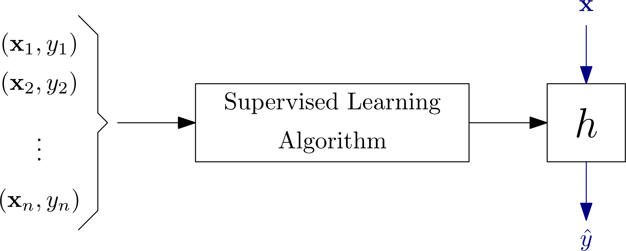
• Given: A training set of $N$ input-output pairs
  $\boxed{\mathcal{D} = \{(\mathbf{x}_1, y_1), (\mathbf{x}_2, y_2), \ldots, (\mathbf{x}_N, y_N)\}}$

  where each pair was generated by an unknown function $y = f(\mathbf{x})$

• Goal: A supervised learning algorithm finds a function $h : \mathcal{X} \to \mathcal{Y}$ that accepts an input vector $\mathbf{x}$ and returns a predicted output $\hat{y}$

• Hypothesis: The function $h$ serves as an approximation of the true function $f$. It is called a hypothesis.

Usage:
$\boxed{\hat{y} = h(\mathbf{x})}$

The hypothesis $h$ is used to predict an output $\hat{y}$ from an unlabeled input $\mathbf{x}$.

Flow: Training pairs $(\mathbf{x}_1, y_1), (\mathbf{x}_2, y_2), \ldots, (\mathbf{x}_n, y_n)$ → Supervised Learning Algorithm → $h$ → Input $\mathbf{x}$ → Output $\hat{y}$

Example: Handwritten digit recognition

• Training: Given images of handwritten digits with labels (0-9), learn function $h$
• Testing: Use $h$ to predict the digit in a new image

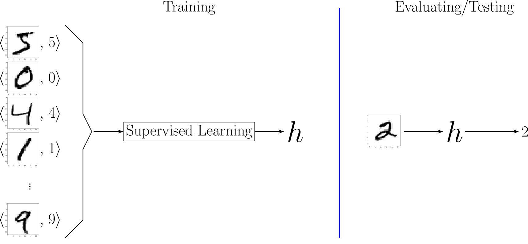
Analogy: Like a teacher showing you labeled examples (this is a 5, this is a 0), and you learn to recognize new examples based on those labeled instances.

2. Unsupervised Learning

Definition: Learning from a set of unlabeled examples ($\{\vec{x_i}\}^N_{i=1}$).

Typical tasks include:

1. Learning a representation function $h : \mathcal{X} \to \mathcal{Z}$ that maps an unlabeled input $\mathbf{x}$ into new representations:
   $z = h(\mathbf{x})$

2. Learning a generative model that captures the joint probability distribution $P(\mathbf{x})$ of the data

   • Examples of generative models:
     • Bayesian Networks: Represent the probabilistic relationships among a set of variables
     • Gaussian Mixture Models (GMMs): Assume that data is generated from a mixture of Gaussian distributions and can capture more complex data distributions than a single Gaussian

Example: Fingerprint representation

• Given a set of fingerprints without labels
  
• Learn a function $h$ that converts a fingerprint into a vector $[z_1, z_2, \ldots]^T$
• GMMs can learn parameters of a mixture of Gaussian distributions that model the data
• The learned parameters can be used to generate new samples that resemble the original data
  
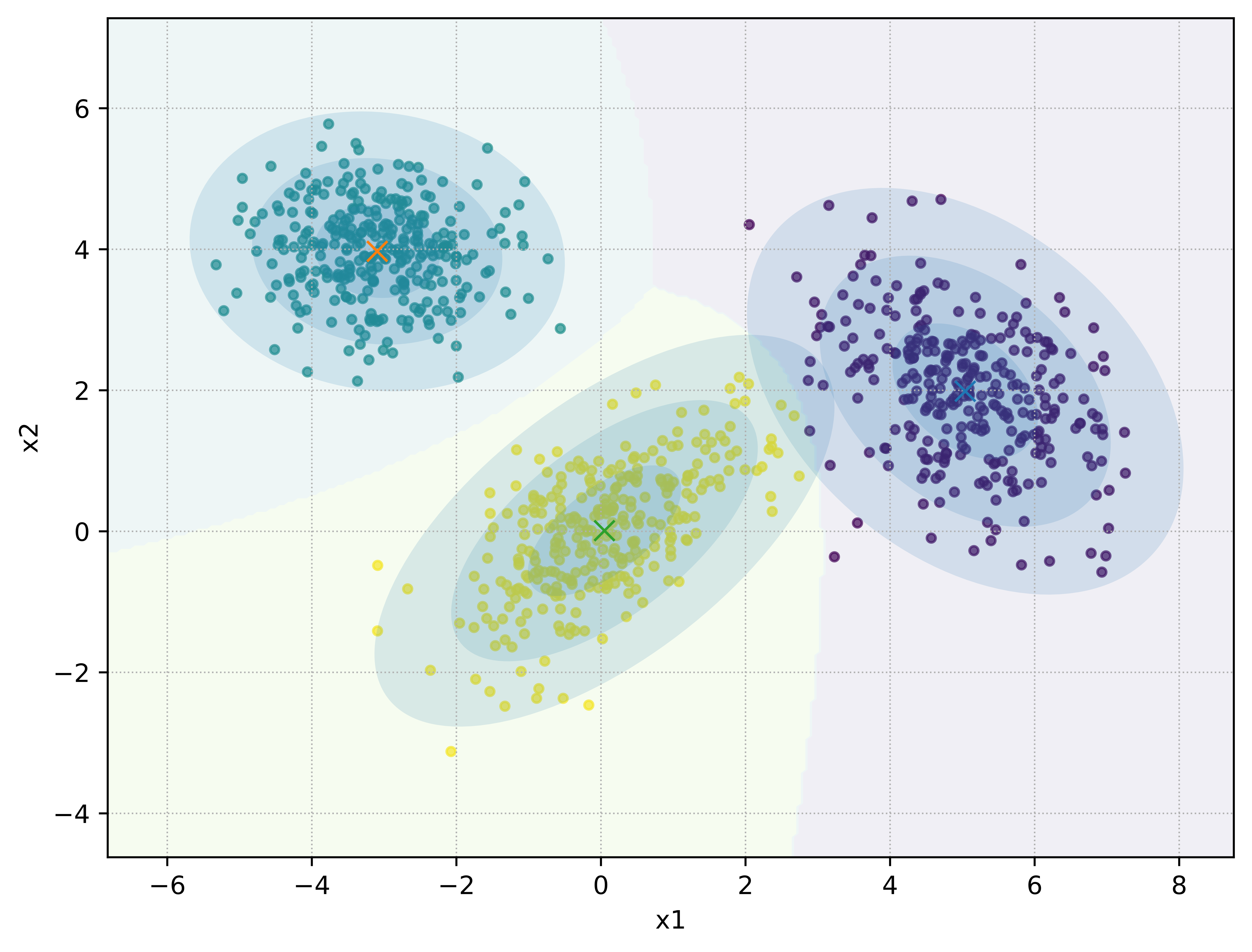
• พอทำมาเป็น cluster, group ๆ แบบนี้สุดท้ายก็ได้ mean, covariance matrix มาเป็นข้อมูลใหม่ ๆ

เราเอา $z$ ที่ได้เนี่ย ไป compare 2 fingerprint ได้ง่าย (easier, more efficient) เช่นว่าแบบ The same มั้ยน้อออออ

Analogy: Like sorting a pile of mixed fruits without anyone telling you what categories to use. You might naturally group them by color, size, or shape - discovering patterns on your own.

3. Reinforcement Learning

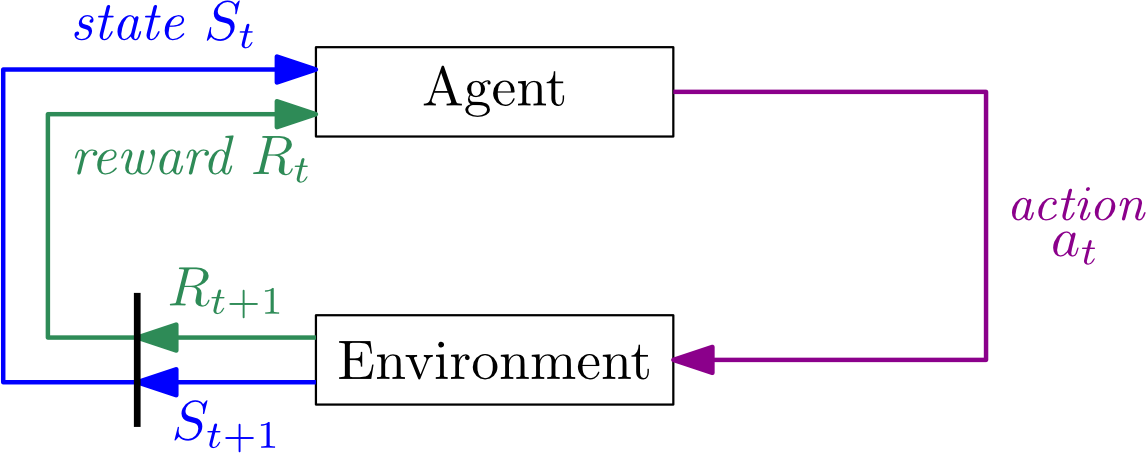
Definition: Learns from interactions with an environment through rewards and penalties.

Process:

• At each time step $t$, the agent receives:
  • Current state $S_t$
  • Reward $R_t$ from the environment
• The agent then selects an action $a_t$ and sends it to the environment
• The environment responds by:
  • Moving to a new state $S_{t+1}$
  • Producing a reward $R_{t+1}$
• The agent uses the observed rewards to update its policy to maximize the expected cumulative future reward

Analogy: Like training a dog - it tries different actions, gets treats (rewards) for good behavior and nothing (or negative feedback) for bad behavior, gradually learning which actions lead to treats.

Example 9.1: Identifying ML Types

Identify whether the following descriptions refer to supervised, unsupervised, or reinforcement learning:

1. Stock price prediction: You have historical data on stock prices, including features such as trading volume, past prices, and other market indicators. The goal is to build a model that predicts the stock price for the next day.
   • Answer: Supervised learning (labeled data with features and target prices)

2. Gene expression dimensionality reduction: You have a high-dimensional dataset containing the expression levels of thousands of genes across various samples. You want to reduce the dimensionality of the data to reveal meaningful patterns that differentiate between different biological states, without any prior knowledge of these states.

   • Answer: Unsupervised learning (no labels, finding patterns)

3. Satellite image object detection: You have a large set of satellite images, some of which are labeled with bounding boxes indicating where objects of interest (e.g., buildings, roads, trees) are located. You need to build a system that can detect and localize objects in new, unseen satellite images.

   • Answer: Supervised learning (labeled with bounding boxes)

4. Self-driving car: A self-driving car must learn to navigate the streets by interacting with its environment. It receives input from sensors like cameras and LiDAR, and its goal is to safely drive from one location to another while avoiding obstacles and following traffic rules. The car continuously adjusts its actions based on rewards (e.g., reaching the destination safely) and penalties (e.g., collisions).

   • Answer: Reinforcement learning (learns through interaction and rewards/penalties)

5. Customer segmentation: You have a collection of customer transaction records, but no labels are provided. Your goal is to group customers into different segments based on their purchasing behavior to better target marketing efforts.

   • Answer: Unsupervised learning (clustering without labels)

6. Table tennis robot: A robot is trained to play table tennis by practicing against human players. It receives a positive reward when it successfully returns the ball and a negative reward when it misses. Over time, it learns to adjust its strategy to maximize successful returns.

   • Answer: Reinforcement learning (learns through rewards/penalties)

9.3 Artificial Neurons

ต่อจากนี้เราจะเรียนเป็น Neural Network แล้วนะ — เริ่มจาก Artificial Neuron เลย เป็น Basic Components connection with AI (เราเอาอันนี้หลาย ๆ ตัวมา connect กันเพื่อ compute complicated task)

Definition: An artificial neuron is a basic computational unit of an artificial neural network. It is inspired by the structure of a biological neuron, but simplified for mathematical modeling.

Process:

1. Takes a set of input values (มาจาก an input vector)
2. Processes them with associated weights and a bias (another scalar value)
3. Applies an activation function to produce an output

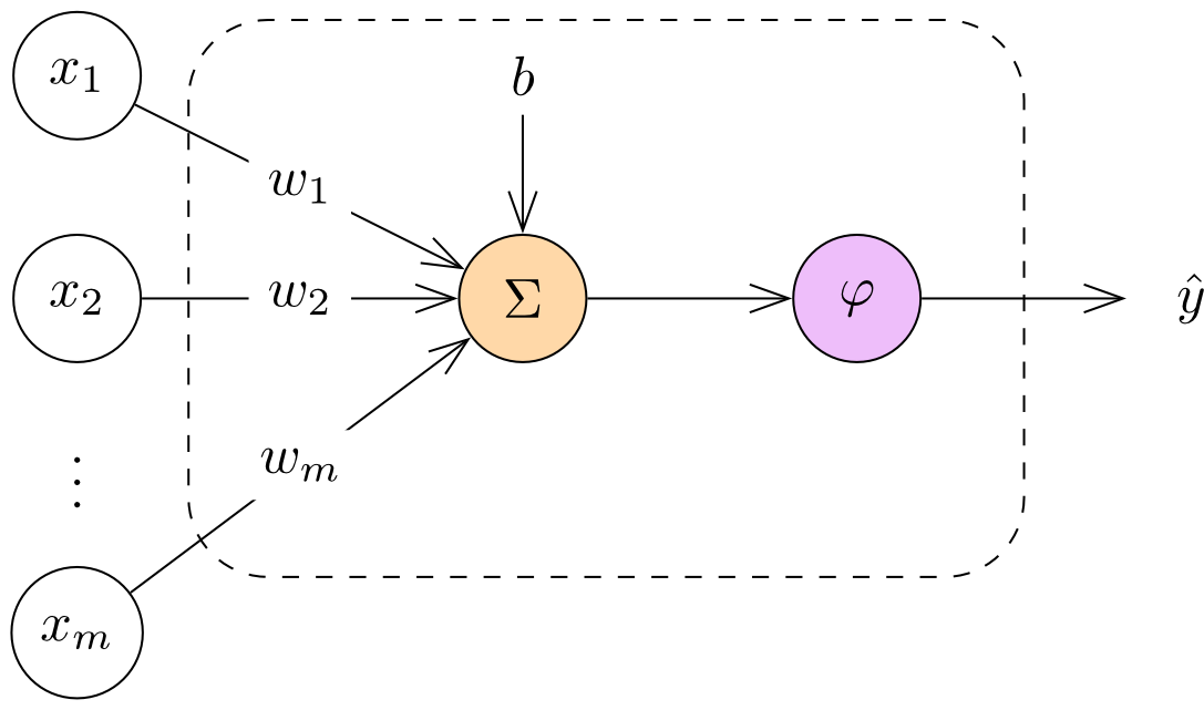
เรารับ Input เข้ามา เสร็จแล้วอาจจะมี Bias value มา แล้วเอามา Calculate เป็น Weighted sum (สีส้ม) หลังจากนั้นก็ส่งไปให้ $\varphi$ (Activation function) → แล้ว Output ออกมาเป็น $\hat{y}$ (a predicted output)

Basic Formulas

Given an input vector $\mathbf{x} = [x_1, x_2, \ldots, x_m]^T$:
$\boxed{z = \Big[\sum_{i=1}^{m} w_i x_i \Big]+ b = \mathbf{w}^T \mathbf{x} + b}\quad\ (9.1)$

มันก็คือ Dot Product ของ Weight Vector กับ $\mathbf{x}$ นั่นแหละ
$\boxed{\hat{y} = \varphi(z)}\quad\ (9.2)$

where:

• $w_i$ = weight of input $x_i$, representing importance of each input
• $b$ = bias, shifting the activation function
• $\varphi(\cdot)$ = activation function
• $\hat{y}$ = predicted output of the neuron

Analogy: Think of a neuron like a decision-maker at a company meeting. Each person (input) speaks, but some voices (weights) carry more influence. The decision-maker adds their own bias, processes all information, and makes a final decision (output).

9.3.1 Activation Functions

The activation function $\varphi(z)$ introduces non-linearity into the neuron's output.

Common activation functions:

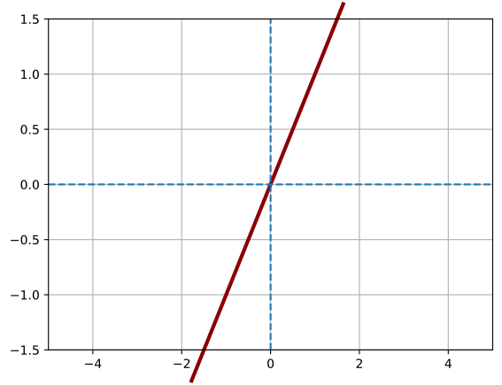
1. Linear Function:
   $\boxed{\varphi(z) = z}$

   • Outputs the input directly
   • Used in regression tasks
     

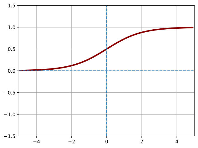
2. Sigmoid Function:
   $\boxed{\varphi(z) = \sigma(z) = \frac{1}{1 + e^{-z}}}$

   • Maps input to a real value between 0 and 1
   • Useful for binary classification
     

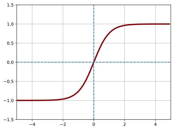
3. Hyperbolic Tangent (tanh):
   $\boxed{\varphi(z) = \tanh(z) = \frac{e^z - e^{-z}}{e^z + e^{-z}}}$

   • Maps input to a real value between -1 and 1
   • Zero-centered, often performs better than sigmoid
   • Also binary classification
     

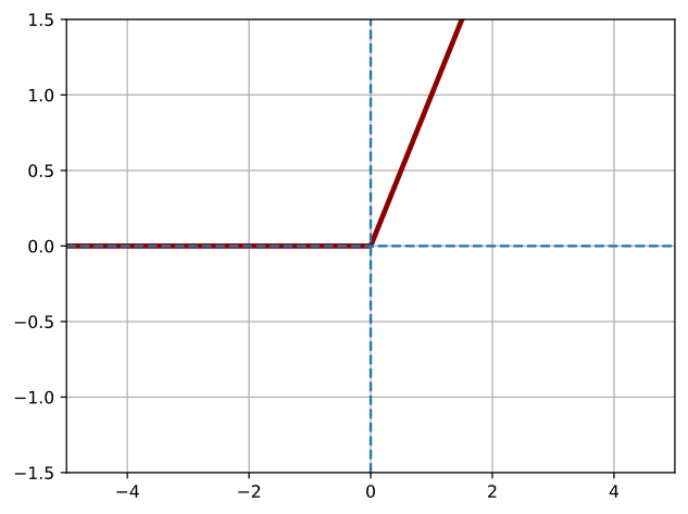
4. Rectified Linear Unit (ReLU):
   $\boxed{\varphi(z) = \text{ReLU}(z) = \max(0, z)}$

   • Outputs 0 for negative inputs
   • Outputs the input itself for positive inputs
   • Most popular in deep learning due to computational efficiency
   • Used in hidden unit of neural network
     

Analogy: Activation functions are like different types of voting systems - linear is proportional voting, sigmoid is binary yes/no, tanh is approval/disapproval, and ReLU is "only count positive votes."

Example 9.2: Neuron Output Calculation

Calculate the output of a neuron with the following parameters:

• Input vector: $\mathbf{x} = [0.5, -1.5, 2.0]^T$
• Weights: $\mathbf{w} = [0.4, 0.6, -0.2]^T$
• Bias: $b = 0.1$
• Activation function: Sigmoid

Solution:
$z = (0.4)(0.5) + (0.6)(-1.5) + (-0.2)(2.0) + 0.1 = 0.2 - 0.9 - 0.4 + 0.1 = -1.0$
$\hat{y} = \sigma(-1.0) = \frac{1}{1 + e^{1.0}} \approx 0.269$

Example 9.3: ReLU Neuron

Calculate the output of a neuron with the following parameters:

• Input vector: $\mathbf{x} = [1.0, -2.0, 0.5, 1.5]^T$
• Weights: $\mathbf{w} = [0.3, 0.2, -0.5, 0.1]^T$
• Bias: $b = 0.4$
• Activation function: ReLU

Solution:
$z = (0.3)(1.0) + (0.2)(-2.0) + (-0.5)(0.5) + (0.1)(1.5) + 0.4$
$z = 0.3 - 0.4 - 0.25 + 0.15 + 0.4 = 0.2$
$\hat{y} = \text{ReLU}(0.2) = \max(0, 0.2) = 0.2$

9.3.2 Artificial Neuron as a Binary Classifier

An artificial neuron can be used as a binary classifier by applying a threshold to its output.

Process:

• If output ≥ threshold → predict one class
• If output < threshold → predict the other class

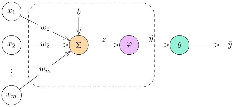
• แนะนำว่า $\varphi$ ควรเป็น Sigmoid or $\tanh$

Formulas:

$\boxed{z = \sum_{i=1}^{m} w_i x_i + b = \mathbf{w}^T \mathbf{x} + b}\quad\ (9.3)$
$\boxed{\hat{y} = \varphi(z)} \quad\ (9.4)$

• แค่เพิ่มมา 1 steps ข้างล่าง
  $\boxed{\tilde{y} = \begin{cases} 1 & \text{if } \hat{y} \geq \theta \\ 0 & \text{if } \hat{y} < \theta \end{cases}} \quad\ (9.5)$

มาจากอนาคต 9.4 Multilayer Perceptrons ถ้ามันอยู่บนเส้นพอดี ก็จะกลายเป็น Class 1 นะ เพราะมีเท่ากับอยู่

where:

• $\theta$ = threshold for classification (e.g., $\theta = 0.5$ for sigmoid, $\theta = 0$ for tanh — เราเลือกเลขที่อยู่ตรงกลาง)
• $\tilde{y}$ = predicted class label (0 or 1 for sigmoid, -1 or 1 for tanh)

Example 9.4: Binary Classification

Problem: A neuron with weights $\mathbf{w} = [0.3, 0.2]^T$, bias $b = -0.3$, and sigmoid activation function is used as a binary classifier with threshold $\theta = 0.5$. Given input vector $\mathbf{x} = [0.7, -0.5]^T$, determine the predicted output $\hat{y}$ and predicted class label $\tilde{y}$.

Solution:
$z = (0.3)(0.7) + (0.2)(-0.5) + (-0.3) = 0.21 - 0.1 - 0.3 = -0.19$
$\hat{y} = \sigma(-0.19) = \frac{1}{1 + e^{0.19}} \approx 0.453$

อย่าลืมว่าเราเอา 0.5 เป็น Threshold
$\tilde{y} = 0 \text{ (since } 0.453 < 0.5\text{)}$

Decision Boundary

Definition: The decision boundary of a binary classifier is the set of points in the input space where the classifier changes its prediction from one class to another.

Decision Boundary of a Sigmoid Unit

For a neuron with sigmoid activation function and threshold $\theta = 0.5$, the decision boundary is defined by:
$\boxed{\sum_{i=1}^{m} w_i x_i + b = 0} \quad\ (9.6)$

• ก็คือ $\sigma(0.5)=0$
  • $w_1x_1+w_2x_2+\dotso+w_mx_m+b=0$
    This is a linear equation in the input space, representing a hyperplane that separates the two classes.

Example 9.5: Decision Boundary Equation

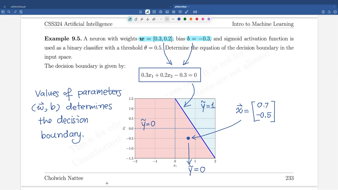
Problem: A neuron with weights $\mathbf{w} = [0.3, 0.2]$, bias $b = -0.3$, and sigmoid activation function is used as a binary classifier with threshold $\theta = 0.5$. Determine the equation of the decision boundary in the input space.

Solution:
The decision boundary is given by:
$0.3x_1 + 0.2x_2 - 0.3 = 0$

Or in slope-intercept form:
$x_2 = -1.5x_1 + 1.5$

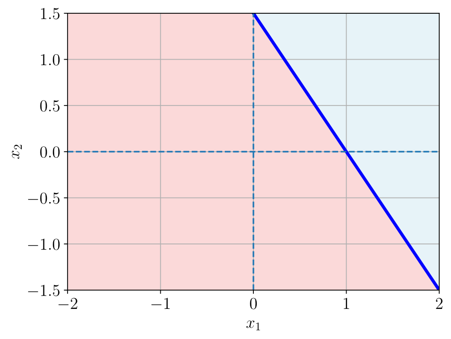
• ฝั่งสีแดง $\tilde{y}=0$
• ฝั่งสีน้ำเงิน $\tilde{y}=1$

9.3.3 Training an Artificial Neuron

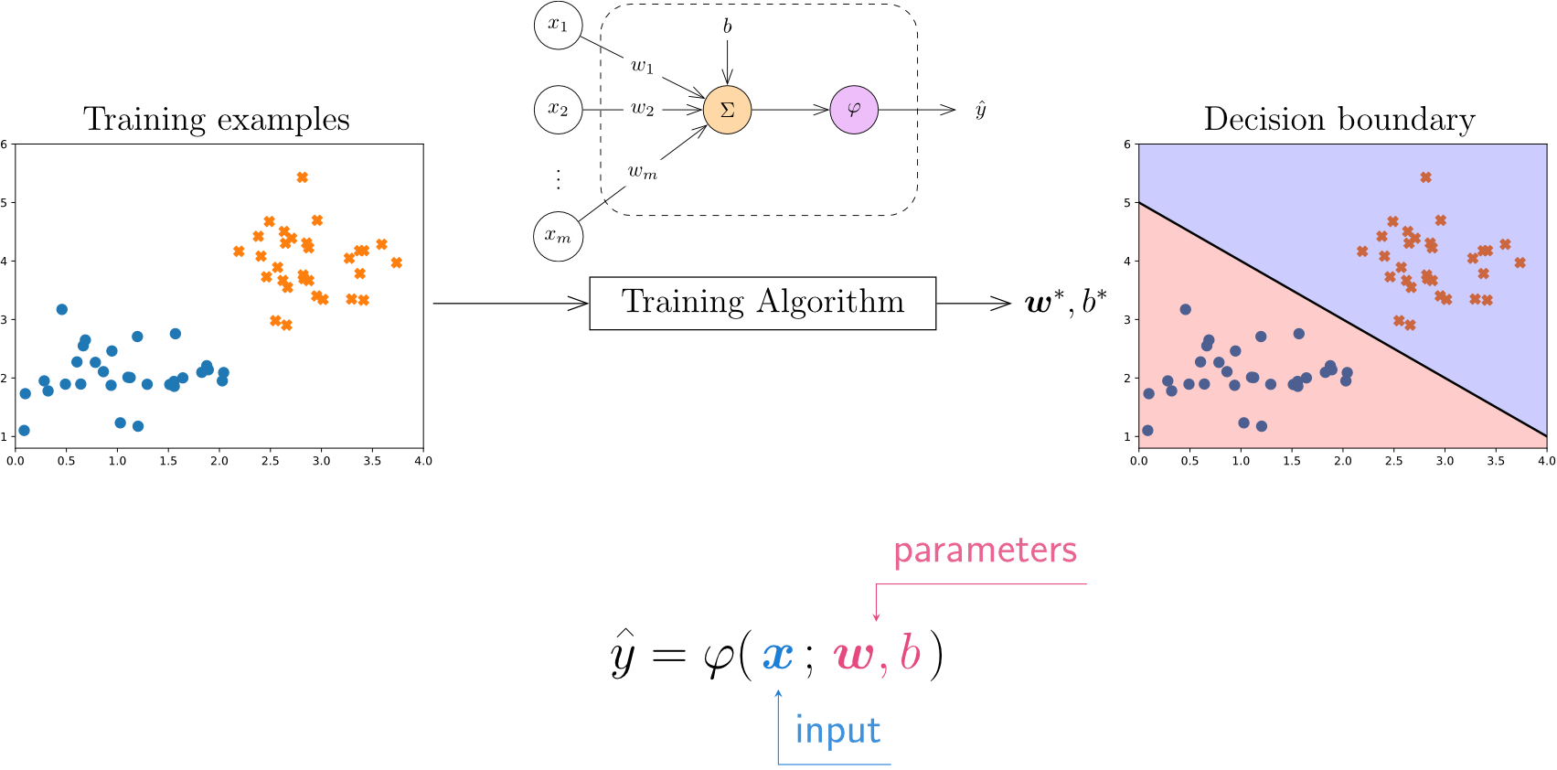
Since the decision boundary of an artificial neuron is determined by its parameter values, training an artificial neuron involves:

• Adjusting its weights and bias
• ==To minimize the error between predicted outputs and actual target values==
• Using a training dataset

Flow: Training examples → Training Algorithm → Optimal parameters $\mathbf{w}^*, b^*$ → Decision boundary

The function with parameters: $\hat{y} = \varphi(\mathbf{x}; \mathbf{w}, b)$

Analogy: Training is like tuning a musical instrument. You adjust the strings (weights and bias) bit by bit, testing the sound (predictions) against the correct notes (true labels) until it sounds right (minimizes error).

แต่สิ่งนี้ก็มี Limitation

9.4 Multilayer Perceptrons

Definition: A multilayer perceptron (MLP) is a type of artificial neural network that consists of multiple layers of neurons, including:

• An input layer
• One or more hidden layers
• An output layer

Why MLPs?

Problem: A single artificial neuron can only represent linear decision boundaries. It cannot model complex, non-linear relationships in data.

Example: The XOR function
$\mathcal{D} = \left\{\left(\begin{bmatrix}0\\0\end{bmatrix}, 0\right), \left(\begin{bmatrix}0\\1\end{bmatrix}, 1\right), \left(\begin{bmatrix}1\\0\end{bmatrix}, 1\right), \left(\begin{bmatrix}1\\1\end{bmatrix}, 0\right)\right\}$
This is a classic example of a problem that ==cannot be represented by a single neuron==.

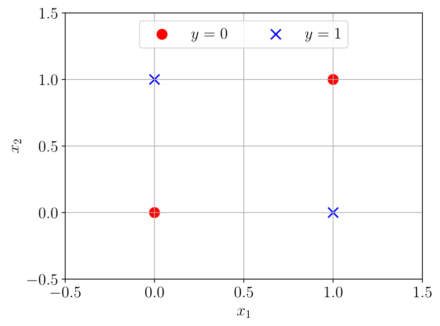
ก็คือบางทีที่มีข้อมูลเป็นแบบนี้อะ มันไม่สามารถแบ่ง/classify แยกออกเป็นสองฝั่งได้ด้วยเส้นตรงเส้นเดียว!!

Analogy: A single neuron is like trying to separate apples from oranges with one straight cut - it works for simple cases. But for complex patterns (like separating mixed fruit salad), you need multiple cuts from different angles (multiple layers).

MLP Computation

Given an input vector $\mathbf{x} = [x_1, x_2, \ldots, x_m]^T$, the output of the $j$-th neuron in layer $l$ is computed as:
$\boxed{z_j^{[l]} = \sum_{i=1}^{n_{l-1}} w_{i,j}^{[l]} a_i^{[l-1]} + b_j^{[l]}}\quad (9.7)$
$\boxed{a_j^{[l]} = \varphi(z_j^{[l]})}\quad (9.8)$

where:

• $n_{l-1}$ = number of neurons in the previous layer $l-1$
• $w_{i,j}^{[l]}$ = weight connecting the $i$-th neuron in layer $l-1$ to the $j$-th neuron in layer $l$
• $b_j^{[l]}$ = bias of the $j$-th neuron in layer $l$
• $a_i^{[l-1]}$ = output of the $i$-th neuron in layer $l-1$, with $a_i^{[0]} = x_i$ for the input layer
• $z_j^{[l]}$ = weighted sum input to the $j$-th neuron in layer $l$
• $a_j^{[l]}$ = output of the $j$-th neuron in layer $l$

Example 9.6: MLP for XOR Problem

Design a multilayer perceptron for the XOR problem.

$\Huge{w_{i,j}^{[l]}}$

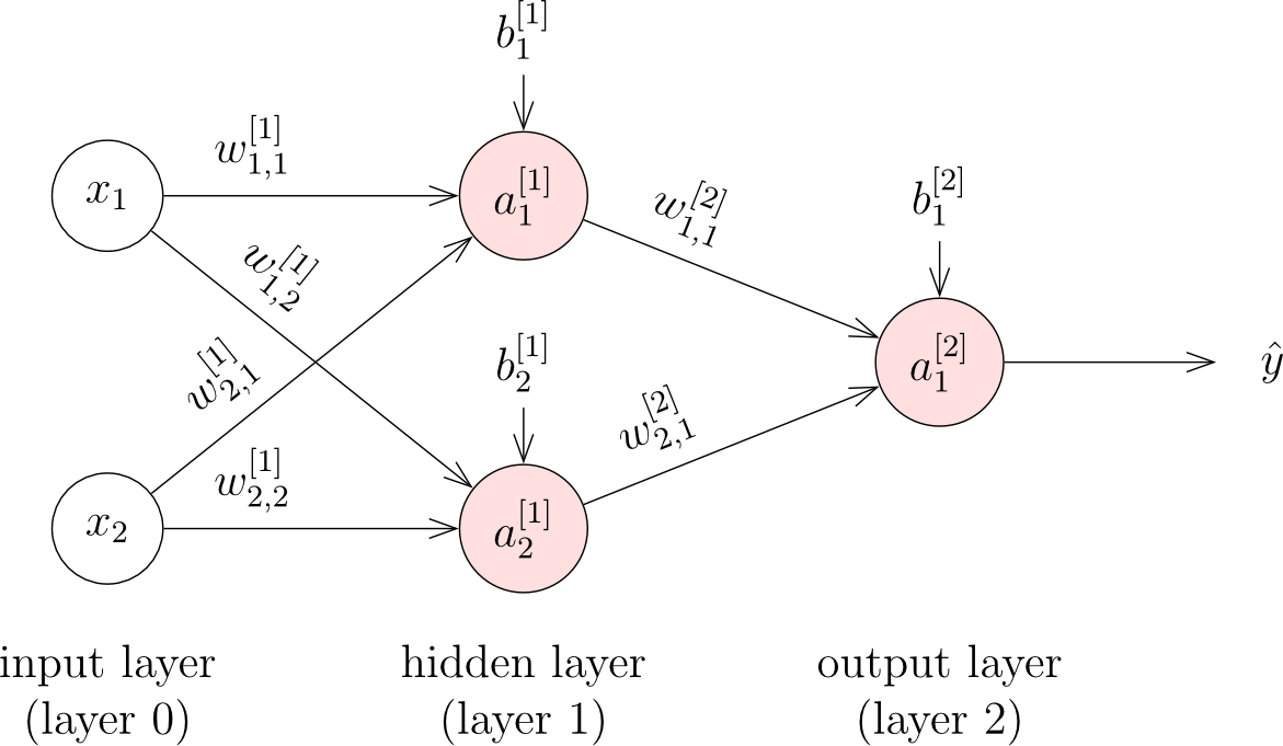
• อ่านได้ว่า Weight from i-th neuron of layer $l-1$ to j-th neuron of layer $l$
  • Superscript represents layer
  • Subscript represents from which unit to which unit

Architecture:

• Input layer (layer 0): $x_1$, $x_2$
  • Input vector: $\mathbf{x}=\begin{bmatrix} x_1 \\ x_2 \end{bmatrix}$
• Hidden layer (layer 1): 2 neurons with sigmoid activation → $a_1^{[1]}$, $a_2^{[1]}$
• Output layer (layer 2): 1 neuron with sigmoid activation → $a_1^{[2]}$ = $\hat{y}$
• All layers are fully connected (อันนี้แปลว่าแต่ละ Layer ไป Connect ตัวต่อไปแบบ every combination possible)

Computation (element-wise):
$z_1^{[1]} = w_{1,1}^{[1]} x_1 + w_{2,1}^{[1]} x_2 + b_1^{[1]}$
$a_1^{[1]} = \sigma(z_1^{[1]})$
$z_2^{[1]} = w_{1,2}^{[1]} x_1 + w_{2,2}^{[1]} x_2 + b_2^{[1]}$
$a_2^{[1]} = \sigma(z_2^{[1]})$
$z_1^{[2]} = w_{1,1}^{[2]} a_1^{[1]} + w_{2,1}^{[2]} a_2^{[1]} + b_1^{[2]}$
$a_1^{[2]} = \sigma(z_1^{[2]})$
$\hat{y} = a_1^{[2]}$
Matrix form:
Layer 1:
$\mathbf{W}^{[1]} = \begin{bmatrix} w_{1,1}^{[1]} & w_{2,1}^{[1]} \\ w_{1,2}^{[1]} & w_{2,2}^{[1]} \end{bmatrix}, \quad \mathbf{b}^{[1]} = \begin{bmatrix} b_1^{[1]} \\ b_2^{[1]} \end{bmatrix}$
Layer 2:
$\mathbf{W}^{[2]} = \begin{bmatrix} w_{1,1}^{[2]} & w_{2,1}^{[2]} \end{bmatrix}, \quad b^{[2]} = b_1^{[2]}$
Forward propagation:
$\mathbf{z}^{[1]} = \mathbf{W}^{[1]} \mathbf{x} + \mathbf{b}^{[1]}$
$\mathbf{a}^{[1]} = \sigma(\mathbf{z}^{[1]})$
$z^{[2]} = \mathbf{W}^{[2]} \mathbf{a}^{[1]} + b^{[2]}$
$\hat{y} = \sigma(z^{[2]})$

Note: $\mathbf{x}$ is a column vector, and $\mathbf{a}^{[1]}$ is also a column vector.

Example 9.7: MLP Output Calculation

Calculate the output of a multilayer perceptron with the following parameters:

• Input vector: $\mathbf{x} = \begin{bmatrix}1\\0\end{bmatrix}$
• Weights and biases:
  $\mathbf{W}^{[1]} = \begin{bmatrix} 1.61 & -2.00 \\ 4.16 & -3.85 \end{bmatrix}, \quad \mathbf{b}^{[1]} = \begin{bmatrix} -0.67 \\ 2.39 \end{bmatrix}$
  $\mathbf{W}^{[2]} = \begin{bmatrix} 3.13 & -3.70 \end{bmatrix}, \quad b^{[2]} = 1.70$
• Activation function: Sigmoid for all neurons

Solution:

Layer 1:
$\mathbf{z}^{[1]} = \begin{bmatrix} 1.61 & -2.00 \\ 4.16 & -3.85 \end{bmatrix} \begin{bmatrix}1\\0\end{bmatrix} + \begin{bmatrix} -0.67 \\ 2.39 \end{bmatrix} = \begin{bmatrix} 0.94 \\ 6.55 \end{bmatrix}$

$\mathbf{a}^{[1]} = \sigma(\mathbf{z}^{[1]}) = \begin{bmatrix} \sigma(0.94) \\ \sigma(6.55) \end{bmatrix} \approx \begin{bmatrix} 0.719 \\ 0.999 \end{bmatrix}$

Layer 2:
$z^{[2]} = \begin{bmatrix} 3.13 & -3.70 \end{bmatrix} \begin{bmatrix} 0.719 \\ 0.999 \end{bmatrix} + 1.70$
$z^{[2]} = 2.251 - 3.697 + 1.70 = 0.254$
$\hat{y} = \sigma(0.254) \approx 0.563$หรือจะตอบได้อีกว่า $\tilde{y}=1$

Visualization of the MLP for XOR

มาโชว์ว่ามันเวิร์คจริง ๆ แล้วนะ กับ Multilayer Perceptron เนี่ย

The hidden layer of the MLP for XOR transforms the input space into a new space where the classes are linearly separable.

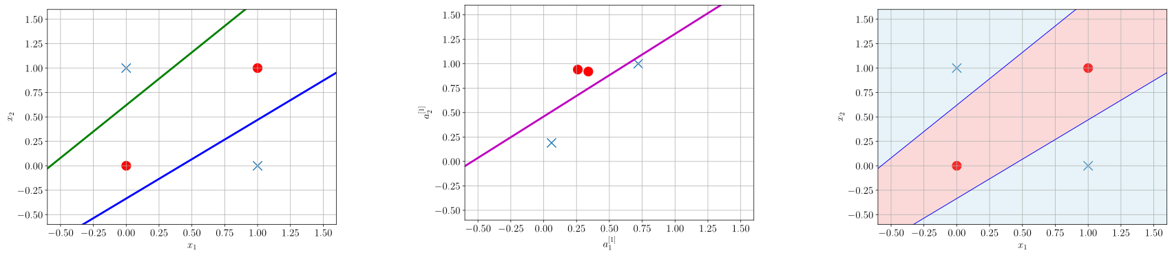
Transformation table:

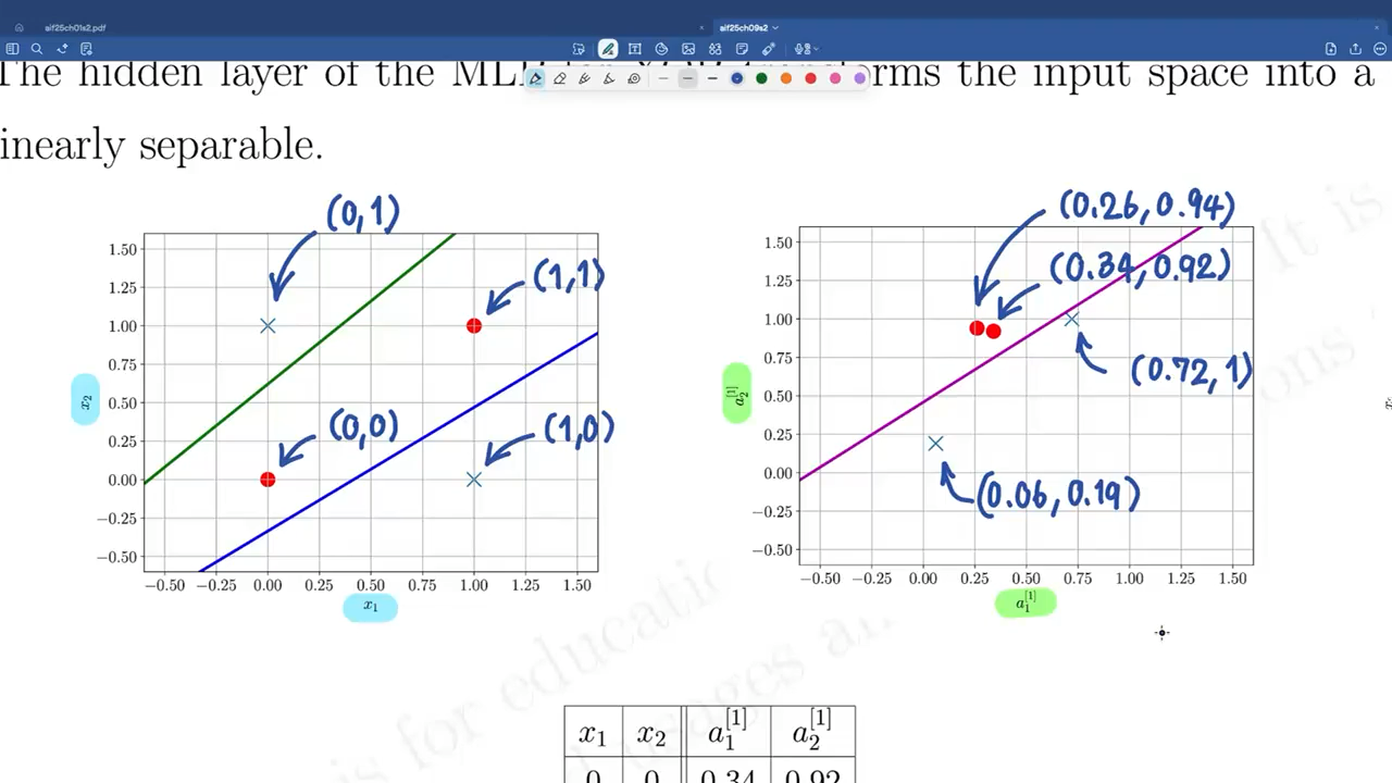
• สุดท้ายก็แบ่งโดยใช้ one line ได้เลยล่ะ

Example 9.8: MLP Architecture Analysis

From the following weights and biases of an MLP, answer the following questions:
$\mathbf{W}^{[1]} = \begin{bmatrix} 1.12 & -3.00 & -1.23 \\ 4.16 & -3.85 & 1.24 \end{bmatrix}, \quad \mathbf{b}^{[1]} = \begin{bmatrix} 1.67 \\ 0.93 \end{bmatrix}$
$\mathbf{W}^{[2]} = \begin{bmatrix} 2.34 & -1.35 \end{bmatrix}, \quad b^{[2]} = -0.97$

All neurons use the sigmoid activation function.

Questions:

1. How many input features does the MLP accept?
   • Answer: 3 (from the number of columns in $\mathbf{W}^{[1]}$)
2. How many neurons are there in the hidden layer?
   • Answer: 2 (from the number of rows in $\mathbf{W}^{[1]}$)
   • ข้อนี้มี 3 layer ไง Layer 0 (input), Layer 1 (hidden), Layer 2 (output)
3. Write down the equations to compute the output of the MLP.
   • Answer:
     $\mathbf{z}^{[1]} = \mathbf{W}^{[1]} \mathbf{x} + \mathbf{b}^{[1]}$
     $\mathbf{a}^{[1]} = \sigma(\mathbf{z}^{[1]})$
     $z^{[2]} = \mathbf{W}^{[2]} \mathbf{a}^{[1]} + b^{[2]}$
     $\hat{y} = \sigma(z^{[2]})$

Number of Parameters in an MLP

The number of parameters (weights and biases) in an MLP can be calculated as:
$\boxed{\text{Total Parameters} = \sum_{l=1}^{L} (n_{l-1} \times n_l + n_l)}\quad (9.9)$
where:

• $L$ = total number of layers (excluding the input layer)
• $n_{l-1}$ = number of neurons in the previous layer $l-1$
• $n_l$ = number of neurons in the current layer $l$

The formula accounts for:

• $n_{l-1} \times n_l$ = weights connecting layer $l-1$ to layer $l$ (สองอันแรก)
• $n_l$ = biases for layer $l$ (อันท้าย ซึ่ง = $\#\text{neurons}$)

Example 9.9: Counting Parameters

Calculate the total number of parameters in an MLP with the following architecture:

• Input layer: 3 neurons
• Hidden layer: 5 neurons
• Output layer: 2 neurons

Solution:

Layer 1 (Input → Hidden):

• Weights: $3 \times 5 = 15$
• Biases: $5$
• Subtotal: $15 + 5 = 20$

Layer 2 (Hidden → Output):

• Weights: $5 \times 2 = 10$
• Biases: $2$
• Subtotal: $10 + 2 = 12$

Total parameters: $20 + 12 = 32$

Using the formula:
$\text{Total} = (3 \times 5 + 5) + (5 \times 2 + 2) = 20 + 12 = 32$

Summary

Key Concepts

1. Machine Learning Types:

   • Supervised: Learn from labeled data
   • Unsupervised: Find patterns in unlabeled data
   • Reinforcement: Learn from rewards and penalties

2. Artificial Neurons:

   • Compute weighted sum: $z = \mathbf{w}^T \mathbf{x} + b$
   • Apply activation: $\hat{y} = \varphi(z)$
   • Can classify with threshold

3. Activation Functions:

   • Linear, Sigmoid, Tanh, ReLU
   • Introduce non-linearity

4. Multilayer Perceptrons:

   • Multiple layers enable non-linear decision boundaries
   • Forward propagation through layers
   • Parameters = weights + biases

Final Analogy: Building an MLP is like constructing a decision-making organization. The input layer receives information, hidden layers are departments that process it from different perspectives, and the output layer makes the final decision based on all processed information.