Produces increasingly accurate approximations to a solution in each iteration
Terminates when the result is sufficiently accurate
Like zooming in on a map - each iteration gets you closer to your exact destination!
Nonlinear Equations in One Dimension
Problem: Given a continuous function f:R→R, find x∗∈R such that f(x∗)=0.
Bolzano's Theorem
Theorem (Bolzano's):
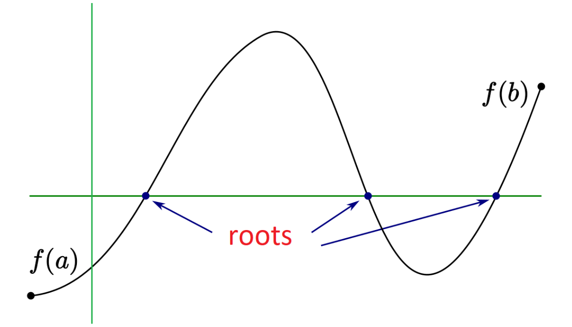
If f is a continuous function on a closed interval [a,b], and f(a) and f(b) differ in sign, then there must be a root within the interval [a,b].
This comes directly from the Intermediate Value Theorem
If you start below the x-axis and end above it (or vice versa), you must have crossed it somewhere!
1. Interval Bisection Method
Setup:
We have two points a and b such that f(a) and f(b) have different signs
By Bolzano's theorem, there is (at least) a root of f in [a,b]
Algorithm:
Let m=a+(b−a)/2 be the midpoint of [a,b]
Evaluate f(m)
Case 1:f(m) has different sign from f(a)
By Bolzano's theorem, there is a root of f in [a,m]
Case 2:f(m) has different sign from f(b)
By Bolzano's theorem, there is a root of f in [m,b]
Repeat until the interval is small enough as required
Like a binary search - you're cutting the search space in half each time!
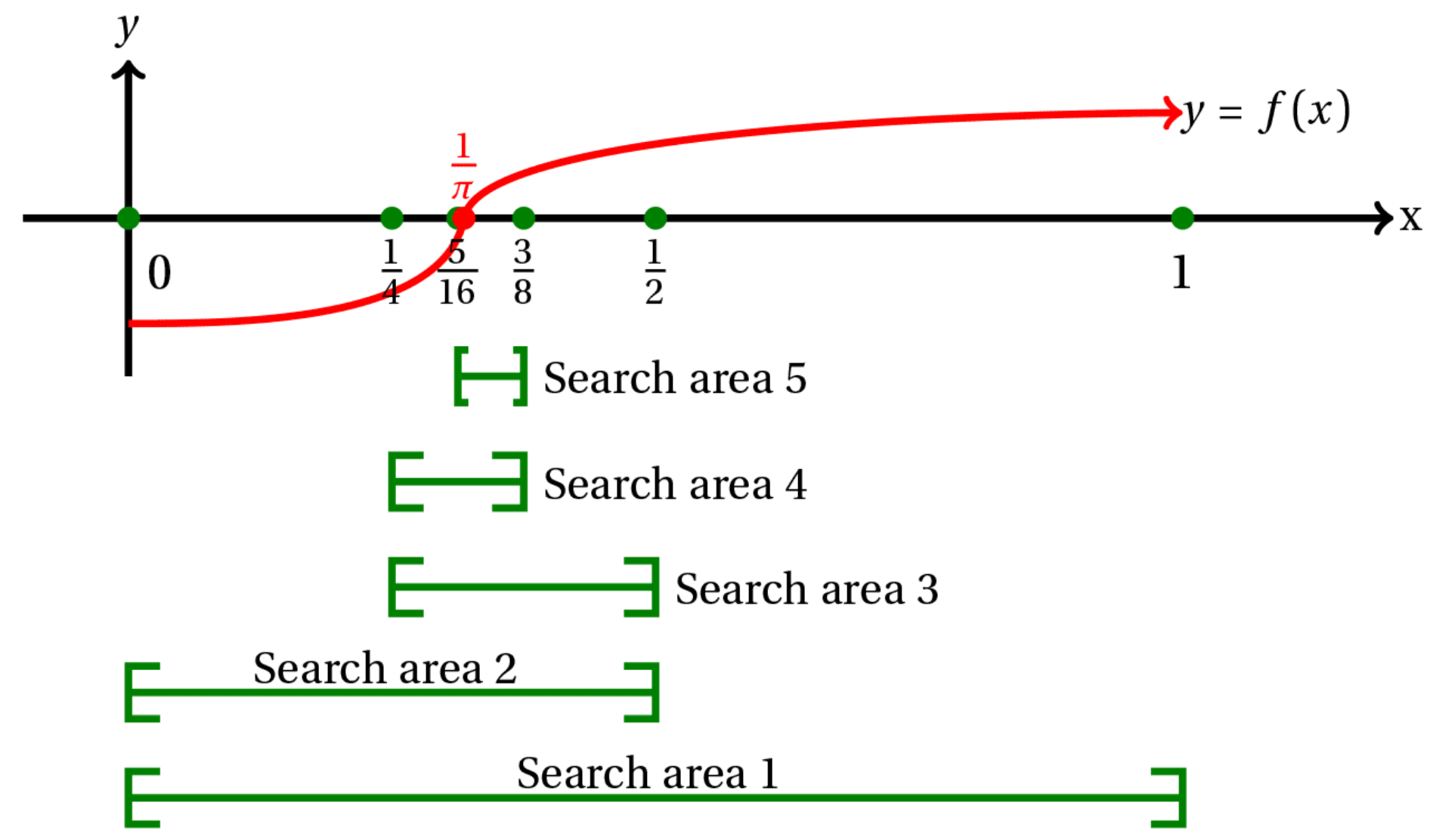
Interval Bisection - Visual Progression
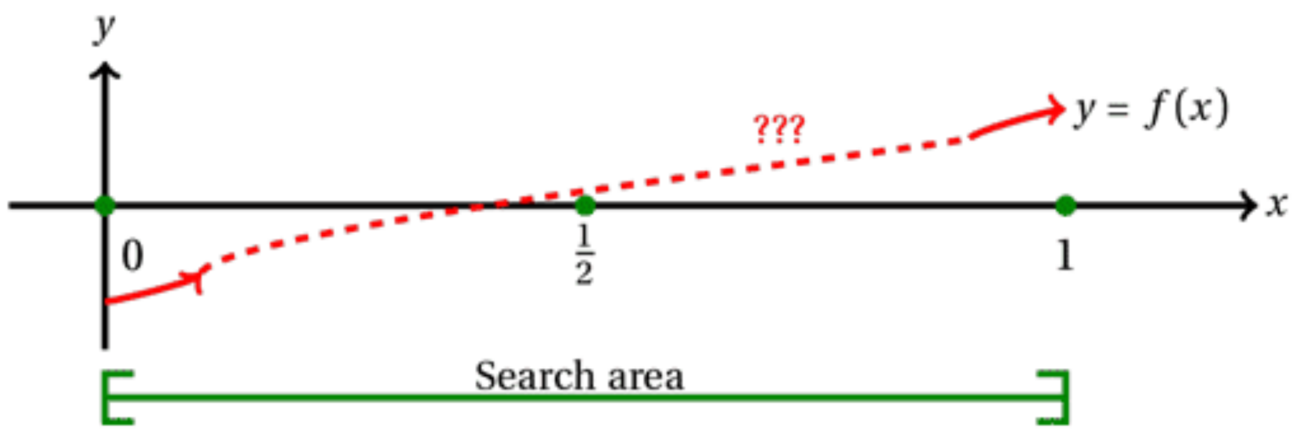
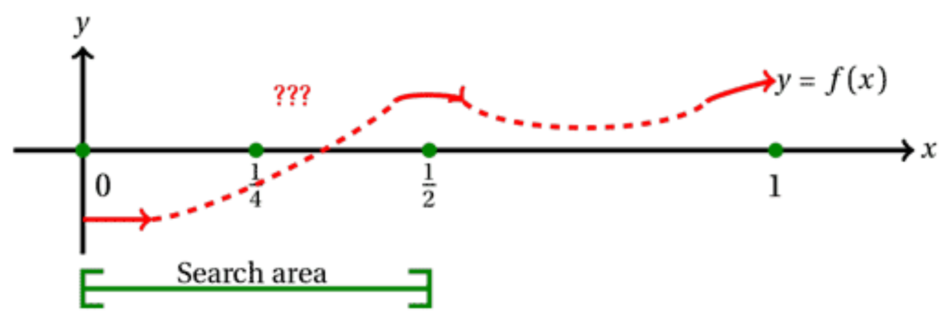
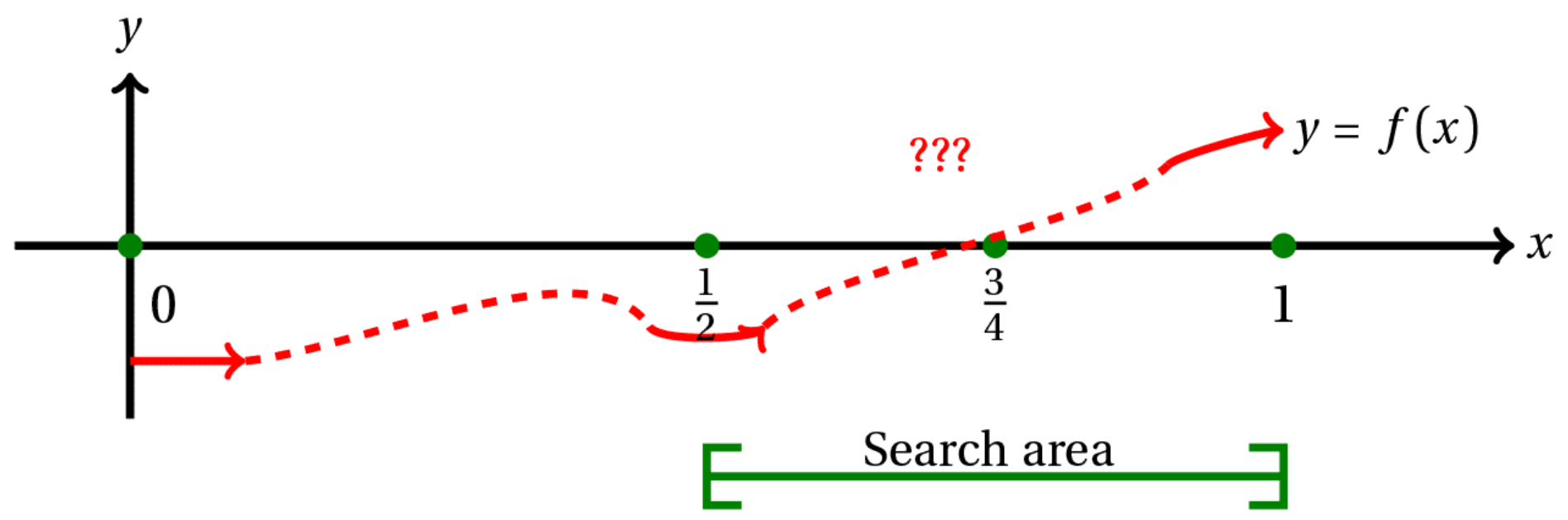
Page 8: Initial search area from 0 to 1, with midpoint at 1/2 Page 9: sign(f(a))= sign(f(m)) - Search area narrows to [0, 1/2] with new midpoint at 1/4 Page 10: sign(f(b))= sign(f(m)) - Search area narrows to [1/2, 1] with new midpoint at 3/4 Page 11: Progressive narrowing shown with multiple search areas:
Search area 1: [0, 1]
Search area 2: narrower interval
Search area 3: even narrower
Search area 4: approaching the root
Search area 5: very close to root (near 1/π)
The root appears to be approximately at x=1/π in the illustration.
Each iteration cuts your uncertainty in half - guaranteed progress!
Pseudocode: Interval Bisection
Initial Setup:
Start with an interval [a,b] such that f(a) and f(b) have different signs
This guarantees a root exists in the interval by the Intermediate Value Theorem
Algorithm:
while ((b - a) > tol) do
    m = a + (b - a)/2          // compute midpoint
    if sign(f(a)) ≠ sign(f(m)) then
        b = m                   // root is in [a, m]
    else
        a = m                   // root is in [m, b]
    end
end
Output:
Optional: Take a point in the final interval (e.g., midpoint) as the approximation
Otherwise: Output the final interval
Analogy: Think of this like playing "hot and cold" to find a hidden object. You keep narrowing down the search area by half each time, always keeping the object within your range.
Implementation Notes
Important Numerical Considerations:
❌ Bad: Computing m = (a + b)/2
Why? Because a + b can overflow for large values
✅ Good: Computing m=a+2(b−a)
This avoids overflow (assuming reasonable initial interval)
How quickly the method converges/ approaches the solution
Definition of Convergence Rate
Notation:
Let x(k) be the approximate solution at iteration k
Let e(k)=x(k)−x∗ (error at iteration k)
Convergence Rate r:
An iterative method converges with rate r if: k→∞lim∥e(k)∥r∥e(k+1)∥=C
for some finite constant C>0.
Classification:
If r=1 and C<1: Linear convergence
If r>1: Superlinear convergence
If r=2: Quadratic convergence
Higher r is better!
Analogy: Think of convergence rate like compound interest. Linear is like simple interest (constant percentage), while quadratic is like compound interest that accelerates dramatically.
Convergence Rate of Interval Bisection
Analysis:
At each iteration, the interval length is reduced by half
The error is at most half the interval length (if using midpoint)
Therefore, error reduces by half each iteration
Result: k→∞lim∥e(k)∥∥e(k+1)∥=0.5
This is linear convergence with r=1 and C=0.5
Interpretation: We gain one additional correct binary bit per iteration
Analogy: Like folding a piece of paper in half repeatedly - each fold gives you exactly half the previous size, very predictable but not super fast.
2. Newton's Method
Derivation (1D Case)
Taylor Series Foundation:
The first two terms of Taylor series give: f(x+h)≈f(x)+f′(x)h The Idea:
Suppose we have x(k) close to a root
We want to find h such that f(x(k)+h)=0
Using the Taylor approximation, solve instead: f(x(k))+f′(x(k))h=0 Solving for h:
f'(x^{(k)})h &= -f(x^{(k)}) \\
h &= -\frac{f(x^{(k)})}{f'(x^{(k)})}
\end{align}$$
**But:** $x^{(k)} + h$ is only an approximation (hopefully better), not a true root.
**Solution:** Repeat the process iteratively!
### Newton's Method Algorithm (1D)
$$\boxed{x^{(k+1)} = x^{(k)} - \frac{f(x^{(k)})}{f'(x^{(k)})}}$$
**Algorithm:**
```
x⁽⁰⁾ = initial guess (a point we hope, close to the solution)
for k = 0, 1, 2, ...
x⁽ᵏ⁺¹⁾ = x⁽ᵏ⁾ - f(x⁽ᵏ⁾)/f'(x⁽ᵏ⁾)
end
```
**Graphical Interpretation:**
Image showing tangent lines at successive points converging to root[]()
![[Pasted image 20251026130448.png|center]]
- At each step, we draw the tangent line at $x^{(k)}$
- The next approximation $x^{(k+1)}$ is where this tangent crosses the x-axis
- The tangent provides a linear approximation that guides us toward the root
> **Analogy:** Like skiing down a hill - at each point, you look at the slope (derivative) and follow it down to get closer to the bottom (root).
### Example 2: Newton's Method
**Problem:** Find a root of $f(x) = x^2 - 3x - 4 = 0$ with $x^{(0)} = 5$
**Setup:**
- $f(x) = x^2 - 3x - 4$
- $f'(x) = 2x - 3$
**Iteration 1:**
$$x^{(1)} = x^{(0)} - \frac{f(x^{(0)})}{f'(x^{(0)})} = 5 - \frac{5^2 - 3(5) - 4}{2(5) - 3} = 5 - \frac{6}{7} = 4.1429$$
**Iteration 2:**
$$x^{(2)} = x^{(1)} - \frac{f(x^{(1)})}{f'(x^{(1)})} = 4.1429 - \frac{(4.1429)^2 - 3(4.1429) - 4}{2(4.1429) - 3} = 4.0039$$
**Iteration 3:**
$$x^{(3)} = x^{(2)} - \frac{f(x^{(2)})}{f'(x^{(2)})} = 4.0039 - \frac{(4.0039)^2 - 3(4.0039) - 4}{2(4.0039) - 3} = 4$$
**Iteration 4:**
$$x^{(4)} = x^{(3)} - \frac{f(x^{(3)})}{f'(x^{(3)})} = 4 - \frac{4^2 - 3(4) - 4}{2(4) - 3} = 4$$
**Note:** When $x^{(k)}$ is a root, $x^{(k+1)} = x^{(k)}$ always because $f(x^{(k)}) = 0$
> **Observation:** Newton's method converged in just 3 iterations (compared to many more for bisection), demonstrating its superior convergence rate!
![[CSS322_Doable_L11_Ex2.pdf]]
### Properties of Newton's Method
**Convergence Behavior:**
1. **Quadratic Convergence (Best Case):**
- If $x^{(0)}$ is close enough to a **simple root**
- Newton's method converges quadratically
- This means the number of correct digits roughly doubles each iteration!
2. **Slower/No Convergence (Problematic Cases):**
- If $x^{(0)}$ is too far from the root
- May converge slowly or may not converge at all
3. **Singular Roots (Problem Case):**
- A **singular root** is $x^*$ where $f'(x^*) = 0$
- Newton's method generally:
- Does not converge to singular roots, OR
- Converges very slowly (linear convergence at best)
> **Analogy:** Newton's method is like a race car - incredibly fast under good conditions (near the root), but can spin out or struggle on rough terrain (far from root or singular roots).
### Example: Singular Root Case
**Problem:** Apply Newton's method to $f(x) = (x - 1)^3 = 0$ with $x^{(0)} = 1.01$
**Analysis:**
- True root: $x^* = 1$
- $f'(x) = 3(x - 1)^2$
- $f'(1) = 0$ → This is a **singular root**!
**Iterations:**
- $x^{(1)} = 1.01 - \frac{(1.01 - 1)^3}{3(1.01 - 1)^2} = 1.0067$
- $x^{(2)} = 1.0067 - \frac{(1.0067 - 1)^3}{3(1.0067 - 1)^2} = 1.0044$
- $x^{(3)} = 1.0030$
- $x^{(4)} = 1.0020$
- $x^{(5)} = 1.0013$
- ...
- $x^{(13)} = 1.0001$
**Observation:**
- Takes more than 13 iterations to get close, despite starting very near the root!
- This problem is actually **[[5 - Conditioning and Stability|ill-conditioned]]**
- มันก็โอเคที่ Newton Method จะไม่ work สำหรับ ill-condition problem เพราะยังไงเราก็ guarantee accurate solution จาก ill-condition problem ไม่ได้อยู่แล้ว
- The slow convergence is inherent to the problem, not just the method
> **Analogy:** Like trying to find the exact top of a perfectly flat mountain - even small measurement errors make it hard to pinpoint the exact peak.
___
## 3. Secant Method
>ต่อยอดมาจาก Newton Method
### Motivation
**Drawback of Newton's Method:**
- Must evaluate both $f(x^{(k)})$ AND $f'(x^{(k)})$ at each iteration
- These evaluations can be expensive computationally
**Key Idea:**
Approximate the derivative using [[9 - Numerical Differentiation#Finite Difference|finite difference]]:
$${f'(x^{(k)}) \approx \frac{f(x^{(k)}) - f(x^{(k-1)})}{x^{(k)} - x^{(k-1)}}}$$
**Advantages:**
- $f(x^{(k)})$ and $f(x^{(k-1)})$ need to be evaluated anyway
- No additional function evaluations required!
- No need to compute derivatives analytically
> **Analogy:** Instead of calculating the exact slope at a point (derivative), we estimate it using two nearby points - like approximating a curve's steepness using two hiking trail markers.
### Secant Method Algorithm
$$\boxed{x^{(k+1)} = x^{(k)} - \frac{f(x^{(k)})(x^{(k)} - x^{(k-1)})}{f(x^{(k)}) - f(x^{(k-1)})}}$$
**Algorithm:**
```
x⁽⁰⁾, x⁽¹⁾ = initial guesses (need TWO starting points)
for k = 1, 2, ...
x⁽ᵏ⁺¹⁾ = x⁽ᵏ⁾ - f(x⁽ᵏ⁾)(x⁽ᵏ⁾ - x⁽ᵏ⁻¹⁾)/(f(x⁽ᵏ⁾) - f(x⁽ᵏ⁻¹⁾))
end
```
**Key Differences from Newton's:**
- ==Requires **two** initial guesses instead of one==
- Only **one** new function evaluation per iteration (vs. two for Newton's)
- **Superlinear** convergence (faster than linear, slower than quadratic)
### Example 3: Secant Method
**Problem:** Find a root of $f(x) = x^2 - 3x - 4 = 0$ with $x^{(0)} = 5$, $x^{(1)} = 4.1429$ (เลขพวกนี้ได้มาจากคิด Newton ข้อก่อนหน้า แต่ไม่เกี่ยวกัน)
**Setup:**
- $f(x^{(0)}) = 5^2 - 3(5) - 4 = 6$
- $f(x^{(1)}) = (4.1429)^2 - 3(4.1429) - 4 = 0.7349$
**Iteration 1 (compute $x^{(2)}$):**
$$x^{(2)} = x^{(1)} - \frac{f(x^{(1)})(x^{(1)} - x^{(0)})}{f(x^{(1)}) - f(x^{(0)})}$$
$$x^{(2)} = 4.1429 - \frac{0.7349(4.1429 - 5)}{0.7349 - 6} = 4.0233$$
**Iteration 2:**
- $f(x^{(2)}) = (4.0233)^2 - 3(4.0233) - 4 = 0.1169$
- **Note:** $f(x^{(1)})$ was already computed!
$$x^{(3)} = 4.0233 - \frac{0.1169(4.0233 - 4.1429)}{0.1169 - 0.7349} = 4.0007$$
**Iteration 3:**
$$x^{(4)} = \ldots = 4$$
**Comparison:**
- Newton's method: Reached $x = 4$ in **3 iterations**
- Secant method: Reached $x = 4$ in **4 iterations**
- ==Trade-off: Secant is slightly slower but doesn't need derivative==
![[CSS322_Doable_L11_Ex3.pdf]]
### Secant Method: Summary
**Comparison to Newton's Method:**
| Feature | Newton's Method | Secant Method |
| ------------------------ | ----------------- | ------------------------------- |
| Function evals/iteration | 2 ($f$ and $f'$) | 1 ($f$ only) |
| Initial guesses needed | 1 | 2 |
| Convergence rate | Quadratic ($r=2$) | Superlinear ($r \approx 1.618$) |
| Requires derivative | Yes | No |
**When to use Secant:**
- When computing $f'(x)$ is expensive or difficult
- When you need good performance without derivatives
- When function evaluations are the bottleneck
> **Analogy:** Newton's method is like using GPS for exact directions (needs extra data), while Secant is like navigating with landmarks (uses what you already see).
---
## Systems of Nonlinear Equations
### Problem Statement
**Given:** $f : \mathbb{R}^n \to \mathbb{R}^n$
**Find:** $x \in \mathbb{R}^n$ such that $f(x) = 0$
### The Jacobian Matrix
**Definition:** For $f : \mathbb{R}^n \to \mathbb{R}^m$, the Jacobian is the $m \times n$ matrix:
$$\boxed{\nabla f(x) = \begin{bmatrix}
\frac{\partial f_1}{\partial x_1} & \frac{\partial f_1}{\partial x_2} & \cdots & \frac{\partial f_1}{\partial x_n} \\
\frac{\partial f_2}{\partial x_1} & \frac{\partial f_2}{\partial x_2} & \cdots & \frac{\partial f_2}{\partial x_n} \\
\vdots & \vdots & \ddots & \vdots \\
\frac{\partial f_m}{\partial x_1} & \frac{\partial f_m}{\partial x_2} & \cdots & \frac{\partial f_m}{\partial x_n}
\end{bmatrix}}$$
> **Analogy:** The Jacobian is like a multidimensional slope - it tells you how the output changes in response to changes in each input direction simultaneously.
### Example 4: Computing Jacobians
**Part 1:** Let $f(x) = \begin{bmatrix} x_1^2 x_2 \\ x_1 + 3x_1x_2 \end{bmatrix}$. Compute $\nabla f(x)$.
**Solution:**
$$\nabla f(x) = \begin{bmatrix}
\frac{\partial f_1}{\partial x_1} & \frac{\partial f_1}{\partial x_2} \\
\frac{\partial f_2}{\partial x_1} & \frac{\partial f_2}{\partial x_2}
\end{bmatrix} = \begin{bmatrix}
2x_1x_2 & x_1^2 \\
1 + 3x_2 & 3x_1
\end{bmatrix}$$
**Part 2:** Let $f(x) = \begin{bmatrix} x_1x_2 + x_3 \\ x_1x_3^3 + x_2x_3 \end{bmatrix}$. Compute $\nabla f(x)$.
**Solution:**
$$\nabla f(x) = \begin{bmatrix}
\frac{\partial f_1}{\partial x_1} & \frac{\partial f_1}{\partial x_2} & \frac{\partial f_1}{\partial x_3} \\
\frac{\partial f_2}{\partial x_1} & \frac{\partial f_2}{\partial x_2} & \frac{\partial f_2}{\partial x_3}
\end{bmatrix} = \begin{bmatrix}
x_2 & x_1 & 1 \\
x_3^3 & x_3 & 3x_1x_3^2 + x_2
\end{bmatrix}$$
---
## Newton's Method for Systems
### Derivation
**Taylor Series for Vector Functions:**
$$\boxed{f(x + h) \approx f(x) + \nabla f(x)h}$$
where $x \in \mathbb{R}^n$ and $h \in \mathbb{R}^n$
**Setup:**
- We have $x^{(k)} \in \mathbb{R}^n$ close to a root
- Want to find $h \in \mathbb{R}^n$ such that $f(x^{(k)} + h) = 0$
**Linear Approximation:**
Solve instead: $f(x^{(k)}) + \nabla f(x^{(k)})h = 0$
**Solving for $h$:**
$$\begin{align}
\nabla f(x^{(k)})h &= -f(x^{(k)}) \\
h &= -(\nabla f(x^{(k)}))^{-1} f(x^{(k)})
\end{align}$$
### Newton's Method Algorithm (Systems)
**❌ Poor Implementation:**
$$x^{(k+1)} = x^{(k)} - (\nabla f(x^{(k)}))^{-1} f(x^{(k)})$$
**Why bad?** Computing matrix inverse is expensive and numerically unstable!
**✅ Better Implementation:**
```
x⁽⁰⁾ = initial guess
for k = 0, 1, 2, ...
Solve: ∇f(x⁽ᵏ⁾)h⁽ᵏ⁾ = -f(x⁽ᵏ⁾) for h⁽ᵏ⁾ [Use GEPP]
x⁽ᵏ⁺¹⁾ = x⁽ᵏ⁾ + h⁽ᵏ⁾
end
```
**Key Points:**
- Solve the linear system directly (don't compute inverse!)
- Use Gaussian Elimination with Partial Pivoting (GEPP)
- Each iteration requires one linear system solve
> **Analogy:** Instead of computing the inverse of a transformation, we directly solve for where we want to go - like finding a route directly rather than reversing all possible routes.
### Example 5: Newton's Method for Systems
**Problem:** Solve $\begin{bmatrix} x_1^2 x_2 \\ x_1 + 3x_1x_2 \end{bmatrix} = \begin{bmatrix} 1 \\ 4 \end{bmatrix}$ with $x^{(0)} = \begin{bmatrix} 2 \\ 0 \end{bmatrix}$
**Transform to $f(x) = 0$ form:**
$$f(x) = \begin{bmatrix} x_1^2 x_2 - 1 \\ x_1 + 3x_1x_2 - 4 \end{bmatrix} = \begin{bmatrix} 0 \\ 0 \end{bmatrix}$$
**Jacobian:**
$$\nabla f(x) = \begin{bmatrix} 2x_1x_2 & x_1^2 \\ 1 + 3x_2 & 3x_1 \end{bmatrix}$$
**Iteration 1:**
Solve $\nabla f(x^{(0)})h^{(0)} = -f(x^{(0)})$:
$$\begin{bmatrix} 2(2)(0) & 2^2 \\ 1 + 3(0) & 3(2) \end{bmatrix} \begin{bmatrix} h_1^{(0)} \\ h_2^{(0)} \end{bmatrix} = -\begin{bmatrix} 2^2(0) - 1 \\ 2 + 3(2)(0) - 4 \end{bmatrix}$$
$$\begin{bmatrix} 0 & 4 \\ 1 & 6 \end{bmatrix} \begin{bmatrix} h_1^{(0)} \\ h_2^{(0)} \end{bmatrix} = \begin{bmatrix} 1 \\ 2 \end{bmatrix}$$
**Solve by GEPP:**
$$h^{(0)} = \begin{bmatrix} \frac{1}{2} \\ \frac{1}{4} \end{bmatrix}$$
**Update:**
$$x^{(1)} = x^{(0)} + h^{(0)} = \begin{bmatrix} 2 \\ 0 \end{bmatrix} + \begin{bmatrix} \frac{1}{2} \\ \frac{1}{4} \end{bmatrix} = \begin{bmatrix} \frac{5}{2} \\ \frac{1}{4} \end{bmatrix}$$
**Iteration 2:**
Solve $\nabla f(x^{(1)})h^{(1)} = -f(x^{(1)})$:
$$\begin{bmatrix} 2(\frac{5}{2})(\frac{1}{4}) & (\frac{5}{2})^2 \\ 1 + 3(\frac{1}{4}) & 3(\frac{5}{2}) \end{bmatrix} \begin{bmatrix} h_1^{(1)} \\ h_2^{(1)} \end{bmatrix} = -\begin{bmatrix} (\frac{5}{2})^2(\frac{1}{4}) - 1 \\ \frac{5}{2} + 3(\frac{5}{2})(\frac{1}{4}) - 4 \end{bmatrix}$$
$$\begin{bmatrix} \frac{5}{4} & \frac{25}{4} \\ \frac{7}{4} & \frac{15}{2} \end{bmatrix} \begin{bmatrix} h_1^{(1)} \\ h_2^{(1)} \end{bmatrix} = \begin{bmatrix} -\frac{9}{16} \\ -\frac{3}{8} \end{bmatrix}$$
**Solve by GEPP:**
$$h^{(1)} = \begin{bmatrix} 1.2 \\ -0.33 \end{bmatrix}$$
**Update:**
$$x^{(2)} = x^{(1)} + h^{(1)} = \begin{bmatrix} \frac{5}{2} \\ \frac{1}{4} \end{bmatrix} + \begin{bmatrix} 1.2 \\ -0.33 \end{bmatrix} = \begin{bmatrix} 3.7 \\ -0.08 \end{bmatrix}$$
**Continuing iterations:**
$$\vdots$$
$$x^{(7)} = \begin{bmatrix} 3 \\ 0.11111\ldots \end{bmatrix}$$
**Note:** The system has two solutions:
- $\begin{bmatrix} 3 \\ \frac{1}{9} \end{bmatrix}$ and $\begin{bmatrix} 1 \\ 1 \end{bmatrix}$ WOWWWW ได้คำตอบจริง ๆ อะ
![[CSS322_Doable_L11_Ex5.pdf]]
The initial guess determines which solution Newton's method converges to!
> **Analogy:** Like hiking - depending on which side of the mountain you start, you'll end up in different valleys (different roots).
### Example 6:
#### Problem Statement
**Solve:**
$$\begin{bmatrix} x_1 + 2x_2 - 2 \\ x_1^2 + 4x_2^2 - 4 \end{bmatrix} = \begin{bmatrix} 0 \\ 0 \end{bmatrix}$$
**Initial guess:** $x^{(0)} = \begin{bmatrix} 1 \\ 2 \end{bmatrix}$
#### Solution
**Setup:**
The Jacobian is:
$$\nabla f(x) = \begin{bmatrix} 1 & 2 \\ 2x_1 & 8x_2 \end{bmatrix}$$
**Iteration 1:**
Solve $\nabla f(x^{(0)})h^{(0)} = -f(x^{(0)})$:
$$\begin{bmatrix} 1 & 2 \\ 2(1) & 8(2) \end{bmatrix} \begin{bmatrix} h_1^{(0)} \\ h_2^{(0)} \end{bmatrix} = -\begin{bmatrix} 1 + 2(2) - 2 \\ 1^2 + 4(2^2) - 4 \end{bmatrix}$$
$$\begin{bmatrix} 1 & 2 \\ 2 & 16 \end{bmatrix} \begin{bmatrix} h_1^{(0)} \\ h_2^{(0)} \end{bmatrix} = \begin{bmatrix} -3 \\ -13 \end{bmatrix}$$
**Solve by GEPP:**
$$h^{(0)} = \begin{bmatrix} -1.83 \\ -0.58 \end{bmatrix}$$
**Update:**
$$x^{(1)} = x^{(0)} + h^{(0)} = \begin{bmatrix} 1 \\ 2 \end{bmatrix} + \begin{bmatrix} -1.83 \\ -0.58 \end{bmatrix} = \begin{bmatrix} -0.83 \\ 1.42 \end{bmatrix}$$
**Iteration 2:**
Solve $\nabla f(x^{(1)})h^{(1)} = -f(x^{(1)})$:
$$\begin{bmatrix} 1 & 2 \\ -1.67 & 11.3 \end{bmatrix} \begin{bmatrix} h_1^{(1)} \\ h_2^{(1)} \end{bmatrix} = \begin{bmatrix} 0 \\ -4.72 \end{bmatrix}$$
**Solve by GEPP:**
$$h^{(1)} = \begin{bmatrix} 0.64 \\ -0.32 \end{bmatrix}$$
**Update:**
$$x^{(2)} = x^{(1)} + h^{(1)} = \begin{bmatrix} -0.83 \\ 1.42 \end{bmatrix} + \begin{bmatrix} 0.64 \\ -0.32 \end{bmatrix} = \begin{bmatrix} -0.19 \\ 1.1 \end{bmatrix}$$
**Continuing iterations eventually converge to solution:**
$$x^* = \begin{bmatrix} 0 \\ 1 \end{bmatrix}$$
---
## Secant Updating Methods for Systems
### Motivation
**The Challenge:**
- The Jacobian has $n^2$ entries
- Approximating it with finite difference formulas requires many additional function evaluations
- This becomes very expensive for large systems
**The Solution:**
- Just like the 1D case, avoid computing the Jacobian by approximating it using previously known values
- Update the Jacobian approximation instead of computing it from scratch
**Broyden's Method:**
- One of the simplest and most effective secant updating methods
- Named after Charles George Broyden
- Provides a good balance between efficiency and effectiveness
> **Analogy:** Instead of taking a fresh survey every time (computing full Jacobian), we update our previous survey with new information (secant update) - much more efficient!
---
## 4. Broyden's Method
### Algorithm
$$\boxed{\text{Broyden's Update: } B^{(k+1)} = B^{(k)} + \frac{(y^{(k)} - B^{(k)}h^{(k)})(h^{(k)})^T}{(h^{(k)})^T h^{(k)}}}$$
**Full Algorithm:**
```
x⁽⁰⁾ = initial guess
B⁽⁰⁾ = initial Jacobian approximation
for k = 0, 1, 2, ...
Solve: B⁽ᵏ⁾h⁽ᵏ⁾ = -f(x⁽ᵏ⁾) for h⁽ᵏ⁾ // Newton-like step
x⁽ᵏ⁺¹⁾ = x⁽ᵏ⁾ + h⁽ᵏ⁾ // Update position
y⁽ᵏ⁾ = f(x⁽ᵏ⁺¹⁾) - f(x⁽ᵏ⁾) // Function change
B⁽ᵏ⁺¹⁾ = B⁽ᵏ⁾ + (y⁽ᵏ⁾ - B⁽ᵏ⁾h⁽ᵏ⁾)(h⁽ᵏ⁾)ᵀ / (h⁽ᵏ⁾)ᵀh⁽ᵏ⁾ // Update Jacobian
end
```
### The Theory Behind Broyden's Update
**Secant Equation:**
We want $B^{(k+1)}$ (approximation of $\nabla f(x^{(k+1)})$) to satisfy:
$$\boxed{B^{(k+1)}(x^{(k+1)} - x^{(k)}) = f(x^{(k+1)}) - f(x^{(k)})}$$
This is the multidimensional generalization of the secant condition.
**The Problem:**
- The secant equation is **underdetermined** - it has many solutions
- We need a way to choose the "best" solution
**Broyden's Choice:**
The update formula in equation (3) gives the solution that:
$$\text{minimizes } \|B^{(k+1)} - B^{(k)}\|_F$$
where $\|\cdot\|_F$ is the Frobenius norm.
> **Interpretation:** Among all matrices satisfying the secant equation, choose the one closest to the previous approximation. This ensures smooth, gradual updates rather than wild changes.
> **Analogy:** Like updating a map - you want to incorporate new information while changing as little as possible of what you already know is correct.
### Properties of Broyden's Method
**Initial Jacobian Approximation $B^{(0)}$:**
Several options for choosing $B^{(0)}$:
1. Use the true Jacobian at $x^{(0)}$: $B^{(0)} = \nabla f(x^{(0)})$
2. Use finite difference approximation
3. Simply set $B^{(0)} = I$ (identity matrix) - simplest option
**Computational Cost:**
- **Naive implementation:** Each iteration still needs to solve a linear system for $h^{(k)}$
- Cost: $O(n^3)$ operations per iteration
- **Efficient implementation:** Update a factorization of $B^{(k)}$ instead
- Cost: Only $O(n^2)$ operations per iteration
- Much more practical for large systems!
**Convergence Properties:**
- **Rate:** Superlinear convergence (but not quadratic)
- Faster than linear, slower than Newton's method
- Similar to 1D secant method
- **Practical Performance:** Despite slower convergence rate, often has net reduction in overall cost
- Especially beneficial when $f$ and its derivatives are expensive to evaluate
- Fewer function evaluations can compensate for more iterations
**Advantages over Newton's Method:**
✅ No need to compute Jacobian at each iteration
✅ Fewer function evaluations per iteration
✅ Can be more efficient with smart factorization updates
✅ Good for expensive function evaluations
**Disadvantages compared to Newton's Method:**
❌ Slower convergence rate (superlinear vs quadratic)
❌ May need more iterations to reach same accuracy
❌ Requires more memory to store approximation
> **Analogy:** Broyden's method is like using a student's improving understanding (updated approximation) versus hiring a new expert tutor each time (computing fresh Jacobian). The student learns gradually but you save money on tutors!
### Example 7: Broyden's Method
>แค่เป็น Method ที่มัน Efficient กว่า Secant / Newton แค่นั้น
#### Problem Statement
**Solve the same system as Example 6:**
$$f(x) = \begin{bmatrix} x_1 + 2x_2 - 2 \\ x_1^2 + 4x_2^2 - 4 \end{bmatrix} = \begin{bmatrix} 0 \\ 0 \end{bmatrix}$$
**Initial guess:** $x^{(0)} = \begin{bmatrix} 1 \\ 2 \end{bmatrix}$
**Initial Jacobian:** Use the true Jacobian at $x^{(0)}$ as $B^{(0)}$
a#### Solution
**Initial Setup:**
$$f(x^{(0)}) = \begin{bmatrix} 3 \\ 13 \end{bmatrix}$$
$$B^{(0)} = \nabla f(x^{(0)}) = \begin{bmatrix} 1 & 2 \\ 2 & 16 \end{bmatrix}$$
**Iteration 0 → 1:**
**Step 1: Solve for $h^{(0)}$**
$$B^{(0)}h^{(0)} = \begin{bmatrix} 1 & 2 \\ 2 & 16 \end{bmatrix} h^{(0)} = \begin{bmatrix} -3 \\ -13 \end{bmatrix} = -f(x^{(0)})$$
**Solution:**
$$h^{(0)} = \begin{bmatrix} -1.83 \\ -0.58 \end{bmatrix}$$
**Step 2: Update position**
$$x^{(1)} = x^{(0)} + h^{(0)} = \begin{bmatrix} 1 \\ 2 \end{bmatrix} + \begin{bmatrix} -1.83 \\ -0.58 \end{bmatrix} = \begin{bmatrix} -0.83 \\ 1.42 \end{bmatrix}$$
**Step 3: Compute function change**
$$f(x^{(1)}) = \begin{bmatrix} 0 \\ 4.72 \end{bmatrix}$$
$$y^{(0)} = f(x^{(1)}) - f(x^{(0)}) = \begin{bmatrix} 0 \\ 4.72 \end{bmatrix} - \begin{bmatrix} 3 \\ 13 \end{bmatrix} = \begin{bmatrix} -3 \\ -8.28 \end{bmatrix}$$
**Step 4: Update Jacobian approximation**
Using the Broyden update formula:
$$B^{(1)} = B^{(0)} + \frac{(y^{(0)} - B^{(0)}h^{(0)})(h^{(0)})^T}{(h^{(0)})^T h^{(0)}}$$
$$B^{(1)} = \begin{bmatrix} 1 & 2 \\ 2 & 16 \end{bmatrix} + \begin{bmatrix} 0 & 0 \\ -2.34 & -0.74 \end{bmatrix} = \begin{bmatrix} 1 & 2 \\ -0.34 & 15.3 \end{bmatrix}$$
**Note:** The Jacobian approximation has been updated! Compare:
- $B^{(0)} = \begin{bmatrix} 1 & 2 \\ 2 & 16 \end{bmatrix}$
- $B^{(1)} = \begin{bmatrix} 1 & 2 \\ -0.34 & 15.3 \end{bmatrix}$
**Iteration 1 → 2:**
**Step 1: Solve for $h^{(1)}$**
$$B^{(1)}h^{(1)} = \begin{bmatrix} 1 & 2 \\ -0.34 & 15.3 \end{bmatrix} h^{(1)} = \begin{bmatrix} 0 \\ -4.72 \end{bmatrix} = -f(x^{(1)})$$
**Solution:**
$$h^{(1)} = \begin{bmatrix} 0.59 \\ -0.30 \end{bmatrix}$$
**Note:** This is slightly different from Newton's method result ($h^{(1)} = \begin{bmatrix} 0.64 \\ -0.32 \end{bmatrix}$) because we're using an approximation of the Jacobian!
**Step 2: Update position**
$$x^{(2)} = x^{(1)} + h^{(1)} = \begin{bmatrix} -0.83 \\ 1.42 \end{bmatrix} + \begin{bmatrix} 0.59 \\ -0.30 \end{bmatrix} = \begin{bmatrix} -0.24 \\ 1.120 \end{bmatrix}$$
**Step 3: Compute function change**
$$f(x^{(2)}) = \begin{bmatrix} 0 \\ 1.08 \end{bmatrix}$$
$$y^{(1)} = f(x^{(2)}) - f(x^{(1)}) = \begin{bmatrix} 0 \\ 1.08 \end{bmatrix} - \begin{bmatrix} 0 \\ 4.72 \end{bmatrix} = \begin{bmatrix} 0 \\ -3.64 \end{bmatrix}$$
**Step 4: Update Jacobian approximation**
$$B^{(2)} = \begin{bmatrix} 1 & 2 \\ 1.12 & 14.5 \end{bmatrix}$$
**Progression of Jacobian approximations:**
- $B^{(0)} = \begin{bmatrix} 1 & 2 \\ 2 & 16 \end{bmatrix}$
- $B^{(1)} = \begin{bmatrix} 1 & 2 \\ -0.34 & 15.3 \end{bmatrix}$
- $B^{(2)} = \begin{bmatrix} 1 & 2 \\ 1.12 & 14.5 \end{bmatrix}$
**Convergence:**
Iterations continue until convergence to the solution:
$$x^* = \begin{bmatrix} 0 \\ 1 \end{bmatrix}$$
![[CSS322_Doable_L11_Ex7.pdf]]
### Comparison: Newton's vs Broyden's
**For this example:**
| Iteration | Newton's $x^{(k)}$ | Broyden's $x^{(k)}$ |
| --------- | --------------------------------------------- | --------------------------------------------- |
| 0 | $\begin{bmatrix} 1 \\ 2 \end{bmatrix}$ | $\begin{bmatrix} 1 \\ 2 \end{bmatrix}$ |
| 1 | $\begin{bmatrix} -0.83 \\ 1.42 \end{bmatrix}$ | $\begin{bmatrix} -0.83 \\ 1.42 \end{bmatrix}$ |
| 2 | $\begin{bmatrix} -0.19 \\ 1.1 \end{bmatrix}$ | $\begin{bmatrix} -0.24 \\ 1.12 \end{bmatrix}$ |
**Observations:**
- First iteration is identical (both use true Jacobian at $x^{(0)}$)
- Subsequent iterations differ slightly
- Both converge to $\begin{bmatrix} 0 \\ 1 \end{bmatrix}$
- Broyden's may need a few more iterations but saves on Jacobian computations
> **Key Insight:** Broyden's method "learns" the Jacobian as it goes, gradually improving its approximation with each iteration, rather than computing it exactly each time.
>ในห้องจบแค่นี้ ข้างล่างสรุปเด้อ ไป [[12 - Optimization]] ต่อออ
---
## Advanced Topics Summary
### Method Comparison Table
| Method | Convergence | Cost/Iteration | Best Use Case |
| ---------------------- | ----------- | ------------------------- | -------------------------------------------- |
| **Newton's** | Quadratic | High (compute $\nabla f$) | Derivatives available, need fast convergence |
| **Broyden's** | Superlinear | Medium (update approx) | Derivatives expensive, many variables |
| **Finite Diff Newton** | Quadratic | Very High ($n^2$ evals) | Small systems only |
### Computational Complexity
**Newton's Method per iteration:**
- Compute Jacobian: Depends on problem (could be $O(n^2)$ to $O(n^3)$)
- Solve linear system: $O(n^3)$ with GEPP
- Function evaluation: Problem-dependent
**Broyden's Method per iteration:**
- Update Jacobian approx: $O(n^2)$ with smart implementation
- Solve linear system: $O(n^3)$ naive, $O(n^2)$ with factorization updates
- Function evaluation: Problem-dependent
---
## Final Summary: Systems of Nonlinear Equations
### Key Concepts
1. **Jacobian Matrix**: The multidimensional derivative
- Size: $n \times n$ for system $f: \mathbb{R}^n \to \mathbb{R}^n$
- Contains all first-order partial derivatives
2. **Newton's Method**: Direct extension of 1D case
- Solve $\nabla f(x^{(k)})h^{(k)} = -f(x^{(k)})$
- Update $x^{(k+1)} = x^{(k)} + h^{(k)}$
- Quadratic convergence (when close to simple root)
3. **Broyden's Method**: Secant updating for systems
- Approximates Jacobian instead of computing it
- Updates approximation each iteration
- Superlinear convergence
- More efficient for expensive functions
### Practical Guidelines
**Choose Newton's Method when:**
- ✅ Jacobian is easy/cheap to compute
- ✅ You're close to the solution
- ✅ Quadratic convergence is critical
- ✅ System is small to medium sized
**Choose Broyden's Method when:**
- ✅ Jacobian is expensive to compute
- ✅ Function evaluations are costly
- ✅ System is large
- ✅ You can tolerate slightly slower convergence
**Implementation Tips:**
- ⚠️ Never compute matrix inverses explicitly
- ⚠️ Always solve linear systems using GEPP or factorizations
- ⚠️ Update factorizations when possible (especially in Broyden's)
- ⚠️ Monitor convergence and add stopping criteria
- ⚠️ Consider line search or trust regions for global convergence
### The Big Picture
> **Analogy:** Think of solving systems of nonlinear equations like finding where multiple curved roads intersect. Newton's method is like having a detailed, up-to-date map at every step (expensive but accurate). Broyden's method is like starting with a rough map and gradually correcting it as you explore (cheaper, still effective).
**The Evolution of Methods:**
1. **1D → nD**: Extension requires linear algebra (solving systems, not just division)
2. **Exact → Approximate**: Trade accuracy for efficiency (Newton → Broyden)
3. **Local → Global**: Add safeguards for poor initial guesses (line search, trust regions)
**Remember:**
- All methods are iterative - they approach the solution gradually
- Initial guess matters! Bad guesses can prevent convergence
- There may be multiple solutions - which one you find depends on where you start
- These are local methods - they find nearby roots, not all roots
## Summary Comparison
### Method Characteristics
| Method | Convergence | Evals/Iter | Initial Points | Pros | Cons |
|--------|-------------|------------|----------------|------|------|
| **Bisection** | Linear ($r=1$, $C=0.5$) | 1 | 2 (bracketing) | • Guaranteed convergence<br>• Robust<br>• Simple | • Slow<br>• Needs bracketing interval |
| **Newton's** | Quadratic ($r=2$) | 2 ($f$ and $f'$) | 1 | • Very fast<br>• Few iterations | • Needs derivative<br>• May not converge<br>• Fails for singular roots |
| **Secant** | Superlinear ($r \approx 1.618$) | 1 | 2 | • No derivative needed<br>• Fast | • Slower than Newton's<br>• May not converge |
### When to Use Each Method
**Use Bisection when:**
- Robustness is critical
- You can easily bracket the root
- Function evaluation is cheap
- You need guaranteed convergence
**Use Newton's when:**
- Speed is essential
- You're close to the root
- Computing derivatives is feasible
- You need quadratic convergence
**Use Secant when:**
- Derivatives are hard to compute
- You need better speed than bisection
- Function evaluation is expensive
- Starting close to the root
---
## Important Formulas Summary
### 1D Methods
**Interval Bisection:**
$$\boxed{m = a + \frac{b-a}{2}}$$
**Newton's Method:**
$$\boxed{x^{(k+1)} = x^{(k)} - \frac{f(x^{(k)})}{f'(x^{(k)})}}$$
**Secant Method:**
$$\boxed{x^{(k+1)} = x^{(k)} - \frac{f(x^{(k)})(x^{(k)} - x^{(k-1)})}{f(x^{(k)}) - f(x^{(k-1)})}}$$
### Systems (Newton's)
**Algorithm:**
1. Solve: $\boxed{\nabla f(x^{(k)})h^{(k)} = -f(x^{(k)})}$
2. Update: $\boxed{x^{(k+1)} = x^{(k)} + h^{(k)}}$
**Convergence Rate:**
$$\boxed{\lim_{k \to \infty} \frac{\|e^{(k+1)}\|}{\|e^{(k)}\|^r} = C}$$
---
## Additional Notes
### Stopping Criteria
Common ways to determine when to stop iterating:
1. **Absolute error:** $|x^{(k+1)} - x^{(k)}| < \text{tol}$
2. **Relative error:** $\frac{|x^{(k+1)} - x^{(k)}|}{|x^{(k+1)}|} < \text{tol}$
3. **Residual:** $|f(x^{(k)})| < \text{tol}$
4. **Maximum iterations:** $k > k_{\max}$
### Practical Considerations
**Bisection:**
- Number of iterations for tolerance $\varepsilon$: $n \approx \log_2\left(\frac{b_0 - a_0}{\varepsilon}\right)$
**Newton's:**
- Check if $f'(x^{(k)}) \approx 0$ to avoid division by zero
- Consider line search or trust region methods for global convergence
**Systems:**
- Condition number of Jacobian affects convergence
- Consider using iterative refinement
- Quasi-Newton methods (e.g., Broyden) avoid computing Jacobian
---
## Key Takeaways
1. ✅ **Bisection** is slow but reliable - use when robustness matters most
2. ✅ **Newton's method** is very fast when close to a simple root - quadratic convergence
3. ✅ **Secant method** balances speed and simplicity - good when derivatives are unavailable
4. ⚠️ **Singular roots** cause problems for Newton's and Secant methods
5. ⚠️ **Initial guess** significantly affects convergence for Newton's and Secant
6. 🔧 For systems, **never explicitly compute matrix inverses** - solve linear systems instead
7. 🎯 The **Jacobian** is the multivariable generalization of the derivative
> **Final Analogy:** Root-finding methods are like different GPS navigation modes - bisection is the "safe route" (slow but sure), Newton's is the "fastest route" (quick but may fail), and Secant is the "balanced route" (good compromise).