7 - Interpolation

Problem Definition

• Problem: For given data $(t_i, y_i), i = 1, \ldots, n$, with $t_1 < t_2 < \ldots < t_n$, we seek (want to find) a function $f : \mathbb{R} \to \mathbb{R}$ such that
  $\boxed{f(t_i) = y_i, \quad i = 1, \ldots, n}$
• $f$ is called an interpolating function or an interpolant for the given data

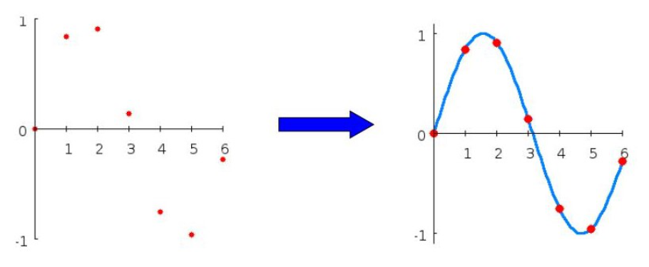
Visual representation: scattered data points → smooth curve that passes through all points

Which Interpolant to Use?

• For a given set of data points, there are infinitely many functions that interpolate it
• Choose the simplest one! (unless we have additional requirements...)
  • แล้วอะไรที่ simplest ล่ะ ก็ polynomial ไงงง

Polynomial Interpolation

• Look for polynomial $f$ that interpolates the data
• Advantages:
  • Simplest and most common interpolation
  • Continuous and differentiable
  • Easy to evaluate
  • Easy to compute its derivatives and antiderivatives

Monomial Basis

• To interpolate $n$ data points, we choose to use a polynomial of degree $n - 1$

• Polynomials in monomial basis:
  $\boxed{p_{n-1}(t) = x_1 + x_2 t + x_3 t^2 + \ldots + x_n t^{n-1}}$

• $x_i$'s are coefficients to be determined

• Often written as:
  $p_{n-1}(t) = \sum_{j=1}^n x_j \phi_j(t)$
  where $\phi_j(t) = t^{j-1}$ are the monomial basis functions

Finding Coefficients of Polynomial Interpolant in Monomial Basis

• Data points: $(t_1, y_1), (t_2, y_2), \ldots, (t_n, y_n)$

• Want $p_{n-1}(t)$ satisfying $p_{n-1}(t_i) = y_i$ for all $i$

• System of equations:

  • $p_{n-1}(t_1) = x_1 + x_2 t_1 + x_3 t_1^2 + \ldots + x_n t_1^{n-1} = y_1$
  • $p_{n-1}(t_2) = x_1 + x_2 t_2 + x_3 t_2^2 + \ldots + x_n t_2^{n-1} = y_2$
  • $\vdots$
  • $p_{n-1}(t_n) = x_1 + x_2 t_n + x_3 t_n^2 + \ldots + x_n t_n^{n-1} = y_n$

• In matrix form:

  1 & t_1 & t_1^2 & \cdots & t_1^{n-1} \\ 1 & t_2 & t_2^2 & \cdots & t_2^{n-1} \\ \vdots & \vdots & \vdots & \ddots & \vdots \\ 1 & t_n & t_n^2 & \cdots & t_n^{n-1} \end{bmatrix} \begin{bmatrix} x_1 \\ x_2 \\ \vdots \\ x_n \end{bmatrix} = \begin{bmatrix} y_1 \\ y_2 \\ \vdots \\ y_n \end{bmatrix}$$

จาก Matrix Form ข้างบน จะ Solve ยังไง เราเรียนมา 5 แบบ:

1. Forward Subtitution 2 - Systems of Linear Equations — ไม่ได้เพราะไม่ใช่ Triangular
2. Backward Substitution
3. Plain GE (Should not be used anymore)
4. GEPP
5. Cholesky 6 - More on Solving Linear Systems ใช้อันไหนดีล่ะ?!!

The Method for Finding Coefficients

• Solve $Ax = y$ for $x$ where:
  • $A$ is the Vandermonde matrix
  • $x$ is the unknown vector of coefficients
  • $y$ is the right-hand side vector
• Algorithm: Use Gaussian Elimination with Partial Pivoting (GEPP)

Important Theorem

ก่อนที่จะใช้ GEPP ได้ต้องเช็คว่าเป็น Non-sigular ก่อน โชคดีที่มี theorem นี้

Theorem: The Vandermonde matrix is nonsingular if the $t_i$'s are all distinct.

Conclusion:

• Consider interpolating $n$ points with polynomial of degree $n - 1$
• If all $t_i$'s are distinct, then polynomial interpolant exists and is unique
• Note: Interpolating with $n - 2$ or lower degree polynomials may not be possible

Example 1

Find polynomial interpolant using monomial basis for: $(-2, -27), (0, -1), (1, 0)$

อย่าลืม - Data points: $(t_1, y_1), (t_2, y_2), \ldots, (t_n, y_n)$

Solution:

• Three points, so $n = 3$
• Use polynomial of degree 2: $p_2(t) = x_1 + x_2 t + x_3 t^2$
  • Degree จะเป็น $n-1=3-1=2$
• System to solve: 1 & t_1 & t_1^2 \\ 1 & t_2 & t_2^2 \\ 1 & t_3 & t_3^2 \end{bmatrix} \begin{bmatrix} x_1 \\ x_2 \\ x_3 \end{bmatrix} = \begin{bmatrix} y_1 \\ y_2 \\ y_3 \end{bmatrix}$$ $$\begin{bmatrix} 1 & -2 & 4 \\ 1 & 0 & 0 \\ 1 & 1 & 1 \end{bmatrix} \begin{bmatrix} x_1 \\ x_2 \\ x_3 \end{bmatrix} = \begin{bmatrix} -27 \\ -1 \\ 0 \end{bmatrix}$$
• Solution: $x = \begin{bmatrix} -1 \\ 5 \\ -4 \end{bmatrix}$
• Interpolating polynomial: $\boxed{p_2(t) = -1 + 5t - 4t^2}$

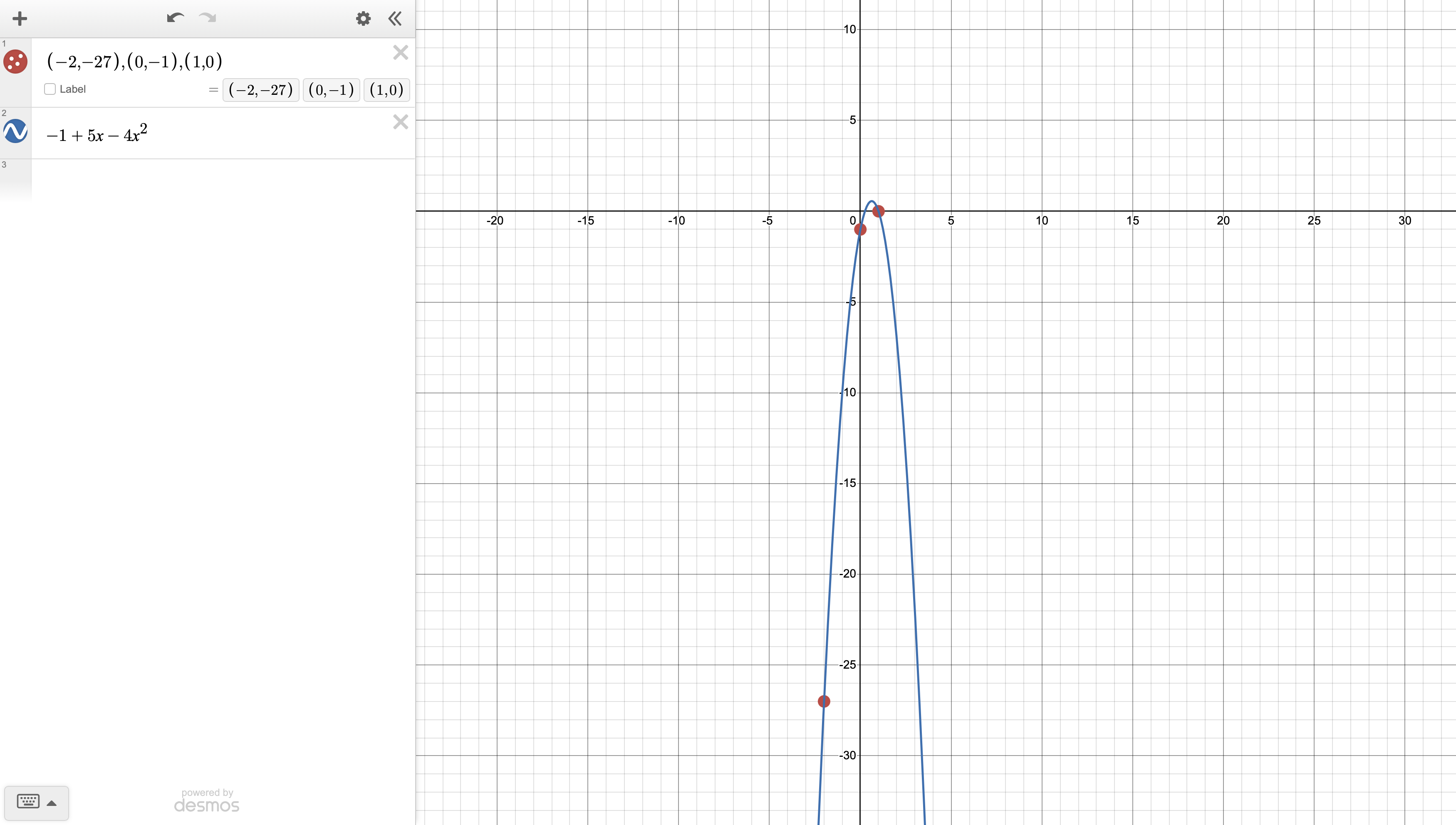
• Verification:
  • $p_2(-2) = -1 + 5(-2) - 4(-2)^2 = -1 - 10 - 16 = -27$ ✅
  • $p_2(0) = -1$ ✅
  • $p_2(1) = -1 + 5 - 4 = 0$ ✅

Example 2 (Exercise)

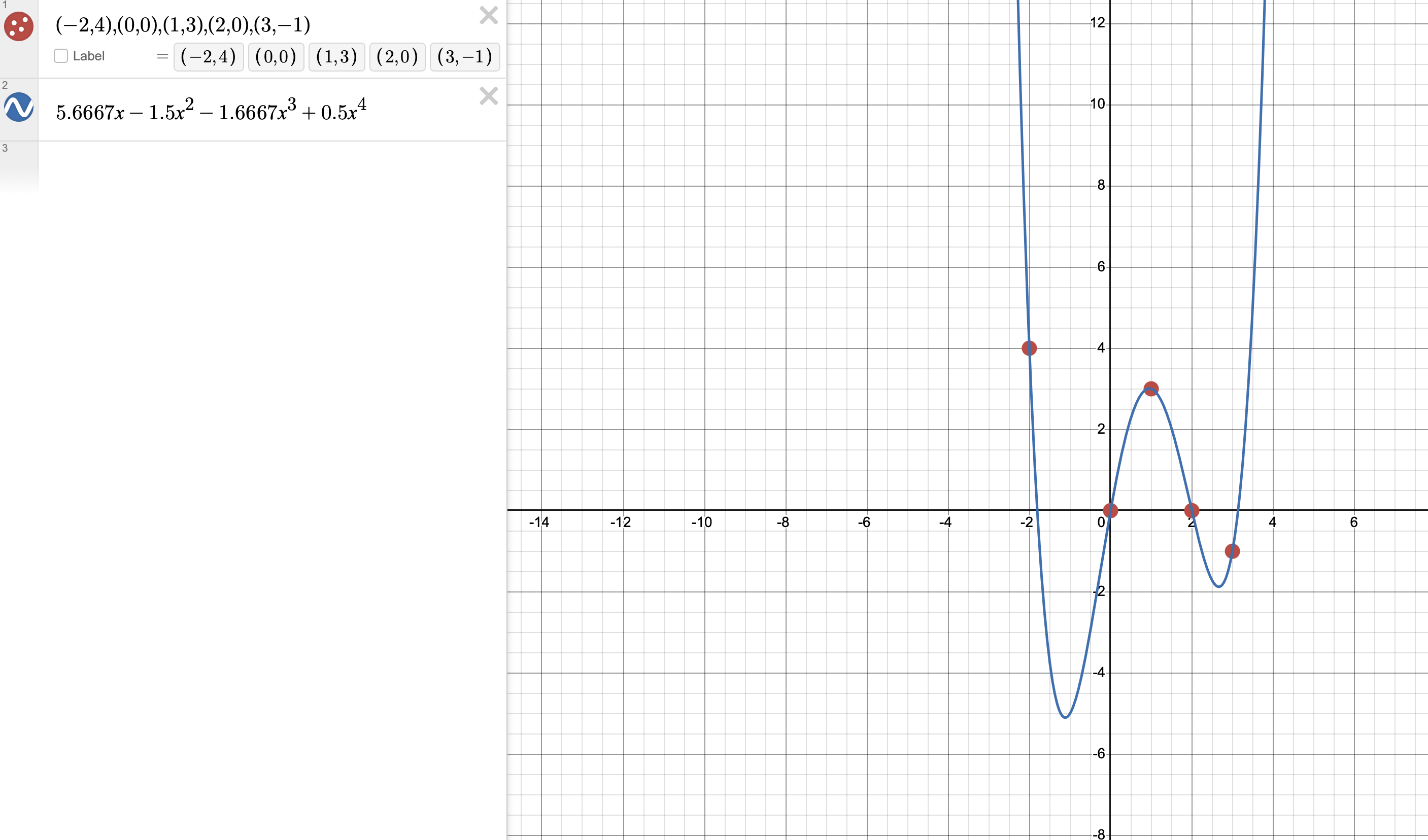
Data points: $(-2, 4), (0, 0), (1, 3), (2, 0), (3, -1)$

Solution:

• Five points, so $n = 5$

• Use polynomial of degree 4: $p_4(t) = x_1 + x_2 t + x_3 t^2 + x_4 t^3 + x_5 t^4$

• System matrix:

  1 & -2 & 4 & -8 & 16 \\ 1 & 0 & 0 & 0 & 0 \\ 1 & 1 & 1 & 1 & 1 \\ 1 & 2 & 4 & 8 & 16 \\ 1 & 3 & 9 & 27 & 81 \end{bmatrix} \begin{bmatrix} x_1 \\ x_2 \\ x_3 \\ x_4 \\ x_5 \end{bmatrix} = \begin{bmatrix} 4 \\ 0 \\ 3 \\ 0 \\ -1 \end{bmatrix}$$

• Solution: $x = \begin{bmatrix} 0 \\ 5.6667 \\ -1.5 \\ -1.6667 \\ 0.5 \end{bmatrix}$

• Interpolating polynomial: $\boxed{p_4(t) = 5.6667t - 1.5t^2 - 1.6667t^3 + 0.5t^4}$

Polynomial Interpolation in MATLAB

>> t = [-2 0 1 2 3];
>> y = [4 0 3 0 -1];
>> p = polyfit(t,y,4)
 
p =
    0.5000   -1.6667   -1.5000    5.6667   -0.0000

• The returned interpolant is $p(1)x^n + p(2)x^{n-1} + \ldots + p(n+1)$
  • ที่ได้ออกมาจะ reverse กับ vector ที่เราทำข้างบน แค่จำไว้ แต่ผลลัพธ์เหมือนกันนั่นแหละ
• Note: You must specify the correct degree for the interpolant, otherwise polyfit() returns something else

Polynomial Evaluation

• Question: How to evaluate a polynomial $p_{n-1}(t) = x_1 + x_2 t + x_3 t^2 + \ldots + x_n t^{n-1}$ at a given point efficiently?

Horner's Method

• Standard form: $p(t) = 2 - t + 3t^2 - 4t^3$

• Horner's form:

  • $p(t) = 2 + t(-1 + 3t - 4t^2)$
  • $p(t) = 2 + t(-1 + t(3 - 4t))$ — Factor it out!!!

• General transformation:
  $p_{n-1}(t) = x_1 + x_2 t + x_3 t^2 + \ldots + x_n t^{n-1} \quad (1)$
  $\downarrow$
  $\boxed{p_{n-1}(t) = x_1 + t(x_2 + t(x_3 + t(\cdots(x_{n-1} + x_n t)\cdots)))} \quad (2)$

• Computational complexity:

  • Evaluating (1): $O(n)$ additions and $O(n^2)$ multiplications
  • Evaluating (2): $O(n)$ additions and $O(n)$ multiplications

Exercise 3: Horner's Rule Examples

1. $5t^4 - 3t^3 + 4t^2 - t + 1$

• Reorder: $1 - t + 4t^2 - 3t^3 + 5t^4$
• Horner's form: $\boxed{1 + t(-1 + t(4 + t(-3 + 5t)))}$

2. $4t^5 - 3t^3 + 2t$

• Fill missing terms: $0 + 2t + 0t^2 - 3t^3 + 0t^4 + 4t^5$
• Horner's form: $\boxed{t(2 + t^2(-3 + 4t^2))}$

Product Notation

• Sigma notation ($\sum$): terms are added together
  $\sum_{i=1}^{10} i^2 = 1^2 + 2^2 + 3^2 + \ldots + 10^2$

• Pi notation ($\prod$): terms are multiplied together
  $\prod_{i=1}^{10} i^2 = 1^2 \cdot 2^2 \cdot 3^2 \cdots 10^2$

• Example: $\prod_{j=4}^7 e^j = e^4 \cdot e^5 \cdot e^6 \cdot e^7$

Lagrange Interpolation

ย้อนกลับไป $p_{n-1}(t) = x_1 + x_2 t + x_3 t^2 + \ldots + x_n t^{n-1}$ คือ Monomial Basis มาดูการเขียนแบบอื่น หรือ basis แบบอื่นบ้างนะ

Lagrange Basis Functions

• Definition: The Lagrange basis functions (a.k.a. fundamental polynomials) are:
  $\boxed{l_j(t) = \frac{\prod_{k=1,k \neq j}^n (t - t_k)}{\prod_{k=1,k \neq j}^n (t_j - t_k)}, \quad j = 1, \ldots, n}$

• Expanded form:

  • $l_1(t) = \frac{(t - t_2)(t - t_3)(t - t_4)\cdots(t - t_n)}{(t_1 - t_2)(t_1 - t_3)(t_1 - t_4)\cdots(t_1 - t_n)}$
  • $l_2(t) = \frac{(t - t_1)(t - t_3)(t - t_4)\cdots(t - t_n)}{(t_2 - t_1)(t_2 - t_3)(t_2 - t_4)\cdots(t_2 - t_n)}$
  • $l_3(t) = \frac{(t - t_1)(t - t_2)(t - t_4)\cdots(t - t_n)}{(t_3 - t_1)(t_3 - t_2)(t_3 - t_4)\cdots(t_3 - t_n)}$
  • $\vdots$
  • $l_n(t) = \frac{(t - t_1)(t - t_2)(t - t_3)\cdots(t - t_{n-1})}{(t_n - t_1)(t_n - t_2)(t_n - t_3)\cdots(t_n - t_{n-1})}$

Properties of Lagrange Basis Functions

• Each $l_j(t)$ is a polynomial of degree $n - 1$
• Key property: 1 & \text{if } i = j \\ 0 & \text{if } i \neq j \end{cases}, \quad i,j = 1, \ldots, n}$$
• Proof:
  • For $i = j$: $l_j(t_j) = \frac{\prod_{k=1,k \neq j}^n (t_j - t_k)}{\prod_{k=1,k \neq j}^n (t_j - t_k)} = 1$
  • For $i \neq j$: $l_j(t_i) = \frac{(t_i - t_1)(t_i - t_2)\cdots(t_i - t_i)\cdots(t_i - t_n)}{\prod_{k=1,k \neq j}^n (t_j - t_k)} = 0$ (due to $(t_i - t_i) = 0$)
• General representation: Any polynomial with degree $n - 1$ can be written as:
  $\boxed{p_{n-1}(t) = \sum_{j=1}^n x_j l_j(t)}$

Finding Coefficients of Polynomial Interpolant in Lagrange Basis

Setup

• Data points: $(t_1, y_1), (t_2, y_2), \ldots, (t_n, y_n)$
• Want: $p_{n-1}(t)$ satisfying $p_{n-1}(t_i) = y_i$ for all $i$
• Write: $\boxed{p_{n-1}(t) = \sum_{j=1}^{n} x_j l_j(t)}$

System of Equations

• $p_{n-1}(t_1) = x_1 l_1(t_1) + x_2 l_2(t_1) + \ldots + x_n l_n(t_1) = y_1$
• $p_{n-1}(t_2) = x_1 l_1(t_2) + x_2 l_2(t_2) + \ldots + x_n l_n(t_2) = y_2$
• $\vdots$
• $p_{n-1}(t_n) = x_1 l_1(t_n) + x_2 l_2(t_n) + \ldots + x_n l_n(t_n) = y_n$

Key Property of Lagrange Basis Functions

$\boxed{l_j(t_i) = \begin{cases} 1 & \text{if } i = j \\ 0 & \text{if } i \neq j \end{cases}}$
for $i, j = 1, \ldots, n$

Solution

• Due to the orthogonal property of Lagrange basis functions:

  • $x_1 l_1(t_1) + x_2 l_2(t_1) + \ldots + x_n l_n(t_1) = x_1 = y_1$
  • $x_1 l_1(t_2) + x_2 l_2(t_2) + \ldots + x_n l_n(t_2) = x_2 = y_2$
  • $\vdots$
  • $x_1 l_1(t_n) + x_2 l_2(t_n) + \ldots + x_n l_n(t_n) = x_n = y_n$

• Therefore: $x_i = y_i$ for all $i$

• Final form: $\boxed{p_{n-1}(t) = y_1 l_1(t) + y_2 l_2(t) + \ldots + y_n l_n(t)}$

Example 4: Lagrange Interpolation

Problem

Find the Lagrange interpolant of the data points $(-2, -27), (0, -1), (1, 0)$.

Solution

• Data points: $(-2, -27), (0, -1), (1, 0)$
• 3 data points → use polynomial of degree 2
• $p_2(t) = y_1 l_1(t) + y_2 l_2(t) + y_3 l_3(t)$
• $p_2(t) = -27 l_1(t) - l_2(t)$ (since $y_3 = 0$)

Lagrange Basis Functions

$l_1(t) = \frac{(t - t_2)(t - t_3)}{(t_1 - t_2)(t_1 - t_3)} = \frac{t(t - 1)}{(-2 - 0)(-2 - 1)} = \frac{t(t - 1)}{6}$
$l_2(t) = \frac{(t - t_1)(t - t_3)}{(t_2 - t_1)(t_2 - t_3)} = \frac{(t + 2)(t - 1)}{(0 + 2)(0 - 1)} = \frac{(t + 2)(t - 1)}{-2}$

Final Result

$p_2(t) = -27 \cdot \frac{t(t - 1)}{6} - \frac{(t + 2)(t - 1)}{-2}$
$p_2(t) = -\frac{27}{6}t(t - 1) + \frac{1}{2}(t + 2)(t - 1)$

Converting to Monomial Basis

$p_2(t) = -\frac{27}{6}t^2 + \frac{27}{6}t + \frac{1}{2}t^2 + \frac{1}{2}t - 1$
$\boxed{p_2(t) = -4t^2 + 5t - 1}$

This matches Example 1 (same interpolant as in monomial basis).

Exercise 5: Four Data Points

Problem

Find the Lagrange interpolant of $(-1, 2), (1, 0), (3, -1), (4, 1)$.

Solution

• 4 data points → use polynomial of degree 3
• $p_3(t) = y_1 l_1(t) + y_2 l_2(t) + y_3 l_3(t) + y_4 l_4(t)$
• $p_3(t) = 2l_1(t) - l_3(t) + l_4(t)$ (since $y_2 = 0$)

Calculations

$l_1(t) = \frac{(t - 1)(t - 3)(t - 4)}{(-1 - 1)(-1 - 3)(-1 - 4)} = \frac{(t - 1)(t - 3)(t - 4)}{-40}$

$l_3(t) = \frac{(t + 1)(t - 1)(t - 4)}{(3 + 1)(3 - 1)(3 - 4)} = \frac{(t + 1)(t - 1)(t - 4)}{-8}$

$l_4(t) = \frac{(t + 1)(t - 1)(t - 3)}{(4 + 1)(4 - 1)(4 - 3)} = \frac{(t + 1)(t - 1)(t - 3)}{15}$

Final Result

$p_3(t) = -\frac{1}{20}(t - 1)(t - 3)(t - 4) + \frac{1}{8}(t + 1)(t - 1)(t - 4) + \frac{1}{15}(t + 1)(t - 1)(t - 3)$

Newton Interpolation

มา Newton Basis บ้างละ55555

Newton Basis Functions

• Can write a polynomial with degree $n - 1$ as:
  $\boxed{p_{n-1}(t) = \sum_{j=1}^{n} x_j \pi_j(t)}$

• Newton basis functions:
  $\boxed{\pi_j(t) = \prod_{k=1}^{j-1} (t - t_k)}$

Explicit Forms

• $\pi_1(t) = 1$ (Newton บอกให้เป็น 1 นะ!)
• $\pi_2(t) = (t - t_1)$
• $\pi_3(t) = (t - t_1)(t - t_2)$
• $\pi_4(t) = (t - t_1)(t - t_2)(t - t_3)$
• $\vdots$
• $\pi_n(t) = (t - t_1)(t - t_2) \cdots (t - t_{n-1})$

Finding Newton Interpolant

General Form

$p_{n-1}(t) = x_1 + x_2(t - t_1) + x_3(t - t_1)(t - t_2) +\ldots + x_n(t - t_1)(t - t_2) \cdots (t - t_{n-1})$

Solving for Coefficients

• For $p_{n-1}(t_1)$: $x_1 = y_1$
• For $p_{n-1}(t_2)$: $x_1 + x_2(t_2 - t_1) = y_2$
• For $p_{n-1}(t_3)$: $x_1 + x_2(t_3 - t_1) + x_3(t_3 - t_1)(t_3 - t_2) = y_3$
• And so on...

Matrix Form