เวลาส่งข้อมูลไรงี้ ข้อมูลมันวิ่งไปถึงปลายทางได้ไง? (เร็วมาก เสี้ยววินาทีเท่านั้นอะ) ทั้ง ๆ ที่อาจจะส่งกันข้ามโลกกก5555 มาดูกันเลยจร้า
Routing in Packet Switching Networks
Core Concept
- Routing is a key function that determines the best path from any source to any destination
- Multiple paths typically exist between nodes
- The "best" path depends on objectives:
- Minimize number of hops
- Minimize end-to-end delay
- Maximize available bandwidth
- Requires global knowledge about network state to perform this task effectively
Analogy: Think of routing like GPS navigation - there are multiple routes from home to work, and the "best" one depends on whether you want the shortest distance, fastest time, or least traffic.
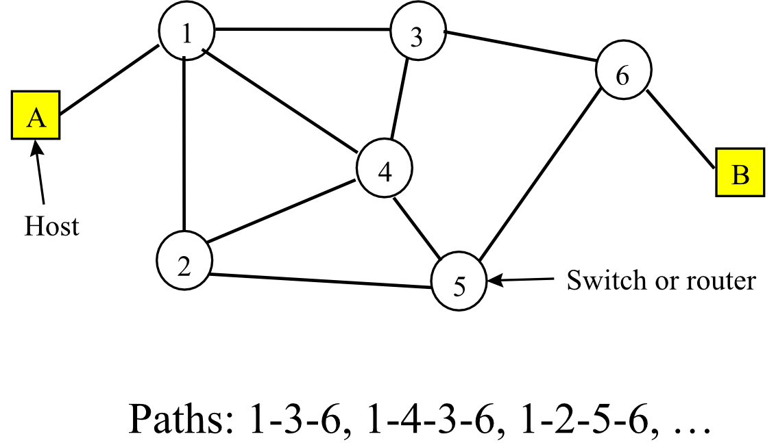
Example Network Structure
หาทางที่ดีที่สุดจากจุด A ไปจุด B
Network Components
- Switches/Routers: Intermediate devices that forward packets
- Hosts: End devices (labeled A, B, C, D)
- Nodes: Numbered 1-6 representing switches/routers
traceroute npwitk.comCriteria for Good Routing Algorithms
What route is the best??? ของจริงมันมีเส้นทางให้เลือกเยอะมาก ระหว่างต้นทางกับปลายทาง ไม่ได้มีถนนเส้นเดียวตรง ๆ แล้วถ้าอยากได้ดี มันดียังไงล่ะ
- Correctness
- Correct route determination
- Accurate delivery of packets
- Robustness (ความทนทาน)
- Adaptive to changes in network topology
- Handles varying traffic load
- ต้องยังทำงานได้ดีอยู่ ไม่ใช่จะล่มไปเลย
- Cleverness
- Ability to detour around congested links
- Determines connectivity of the network
- หลบเลี่ยงเส้นทางที่มีปัญหา
- Efficiency
- Rapid route finding
- Minimization of control messages
- พยายามใช้ทรัพยากรน้อยสุด เช่น Control messages ที่คุยกันระหว่าง router ไม่ให้กิน bandwidth มากเกินไปจนกระทบต่อการส่งข้อมูลของผู้ใช้
Classification of Routing Algorithms
มีหลายประเภทด้วยเลยล่ะ
Static vs. Dynamic
- Static
- Manually computed routes
- Simple implementation
- Not scalable or dynamic
- Dynamic
- Automatic route computation
- Adaptive to network dynamics
- More complicated
Static ก็ตั้งค่าเส้นทางตายตัวไว้เลย ง่ายแต่ไม่ยืดหยุ่น
Dynamic คือ router มันคุยกันเอง คำนวณเส้นทางที่ดีที่สุด ณ เวลานั้น แบบ automatic (ชีวิตจริงใช้อันนี้)
Centralized vs. Distributed
แบ่งตามใครเป็นคนคิดเส้นทางล่ะ
- Centralized
- Central entity computes all routes
- Loads routes into all routers
- Not scalable
- Distributed
- Routers exchange topology information
- Each router performs own route computation
- May have inconsistent or loop routes
- Centralized มีศูนย์กลางคิดให้ทุกอย่างเลย ข้อดี ข้อมูลแม่นยำ ข้อเสีย ถ้าศูนย์กลางล่ม ก็จบเลย5555
- Distributed คือ router แต่ละตัวคิดเอง โดยแลกเปลี่ยนข้อมูลกับเพื่อนบ้าน แต่ต้องคุยกันดี ๆ ไม่งั้นตีกันอีก อาจจะเกิด Loop ได้
Routing by Network Type
- Datagram networks: Routing on packet-by-packet basis
- อันนี้ Router จะตัดสินใจให้ Packet แต่ละตัวแยกกันเลย งั้นแปลว่าส่ง Email รอบนึง แต่ละ Packet อาจจะไปคนละเส้นทางก็ได้
- Virtual Circuit (VC) networks: Routing executed during connection setup
- ต่างออกไป จะหาเส้นทางที่ดีที่สุดแค่ครั้งเดียว ตอน connection setup พอได้แล้ว packet ทั้งหมดของการเชื่อมต่อนั้น ก็จะวิ่งไปทางนั้นตลอด
แล้ว Router มันจำเส้นทางที่มันจองไว้ได้ไง หรือมันเก็บไว้ที่ไหนเหร๋อ?
คำถามถูกต้องเลย มันจะเก็บไว้ใน Routing Tables นั่นเองงง!
Routing Tables
netstat -rnPurpose
หน้าที่เป็น สมุดจด/ป้ายบอกทาง ของ Router นั่นแหละ พอมี Packet วิ่งเข้ามา เดี๋ยวมันจะเปิดดู แล้วรู้ว่าปลายทางนี้ ต้องส่งไปให้ Router ตัวไหน
- Store routing information
- Looked up to forward packets
Format by Network Type
ซึ่ง ๆ หน้าตาตารางของไอ่ 2 Network Types นี้ก็ต่างกันอีกนะ
Datagram Networks
- Destination address + Next hop
ถ้า Destination เป็นตัวนี้ จะต้องส่งต่อไป next hop ไหน แค่นี้เลย
Virtual Circuit Networks
- Incoming VCI + Outgoing VCI + Outgoing port number
ตารางซับซ้อนกว่า: ต้องจำว่า เข้ามาตัวนี้ ต้องส่งไปพอร์ตไหน แล้วเปลี่ยนเป็น Outgoing VCI
Analogy: A routing table is like a train station's schedule board - it tells you which platform (next hop) to go to for your destination.
Virtual-Circuit Packet Switching
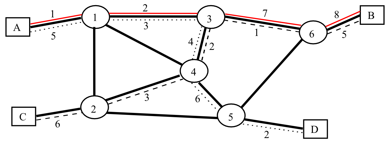
Example Connections
Three channels shown in the example:
- Solid line: A → 1 → 2 → 7 → 8 → B with local VCIs: 1, 2, 7, 8
- Dotted line: A → 5 → 3 → 4 → 6 → 2 → D with local VCIs: 5, 3, 4, 6, 2
- Dashed line: C → 6 → 3 → 2 → 1 → 5 → B with local VCIs: 6, 3, 2, 1, 5
Why Use Local VCIs Instead of Global VCIs?
- Easier searching: Local uniqueness makes finding available VCI simpler
- More capacity: More available local VCIs means more possible connections
VCI คือเลขที่ใช้ในการอ้างอิงการเชื่อมต่อใน Network — แต่ ๆ แทนที่จะใช้เลขเดียวกันตั้งแต่ ต้นทาง ยัน ปลายทาง (Global VCI) ซึ่งจัดการยาก และอาจจะมีไม่พอใช้ จึงนิยมใช้ Local VCI มากกว่า ก็คือ VCI นี้จะมีความหมายเฉพาะในแต่ละ Link หรือ Router สองตัวที่ติดกันเท่านั้น ไปตัวถัดไปเลขก็จะเปลี่ยน
คือพูดง่าย ๆ ถ้าใช้ Local VCI คือมันจะหาเลขมาง่ายกว่า เลขที่ Available อะนะ ไม่ต้องตรวจทั้งระบบว่าเลขมันซ้ำมั้ยอะไรอีก คือในภาพรวมคือใช้ได้เยอะกว่า เพราะไม่ต้องกังวลเรื่องเลขซ้ำ
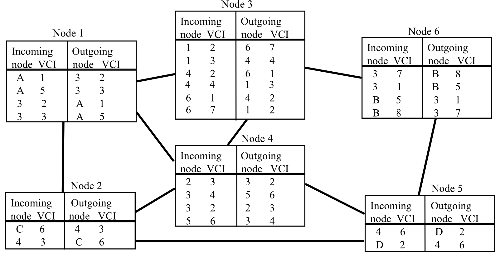
Virtual Circuit Routing Table Structure
Each node maintains a table with:
- Incoming node and Incoming VCI
- Outgoing node and Outgoing VCI
Analogy: Local VCIs are like apartment numbers - each building (node) can have its own apartment 101, making it easier to manage than having globally unique apartment numbers across an entire city.
Datagram Packet Switching
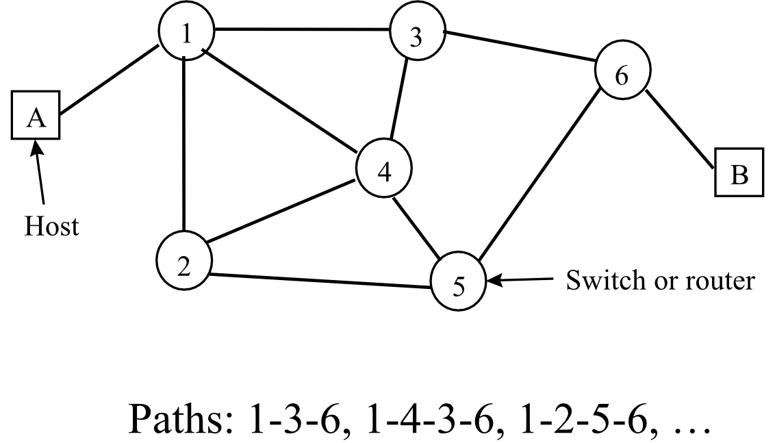
Routing Table Structure
- Each node maintains: Destination → Next node
- Routes packets independently based on destination address
- No connection setup required
Example Routing Tables
For a 6-node network, each node has entries for all other nodes showing which neighbor to forward to.
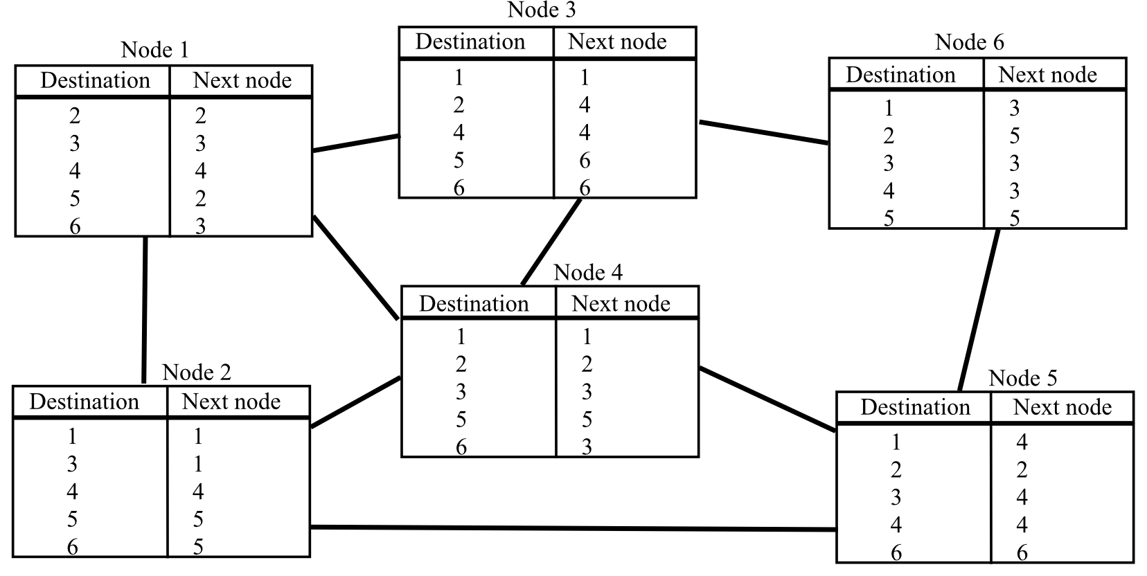
Router ตัวเดียว จะเก็บ Routing Table เส้นทางของทั้งโลกได้ยังไงเอ่ย
นี่เป็นปัญหาจริง ๆ ในทางปฏิบัติเลย ถ้าให้ Router ทุกตัวรู้หมดทุก Host ปลายทาง ตารางจะต้องใหญ่มาก ๆ วิธีแก้คือการใช้ Hierarchical Routing
Hierarchical Routing
Problem
- Routing table size becomes extremely large as network grows
Solution
- Hierarchical addressing: Hosts close together get network addresses with same prefixes
- Remote routing: Treat multiple hosts as one address entry (single entry in routing table)
- Local routing: Hosts treated separately within local area
- Two-stage forwarding:
- Forward to area based on remote routing table
- Forward to specific host based on local routing table
Benefits Illustrated
- Without hierarchy: Need individual entries for every host (e.g., 0000, 0001, 0010, ...)
- With hierarchy: Group hosts (e.g., all hosts starting with 00, 01, 10, 11)
- Dramatically reduces routing table size
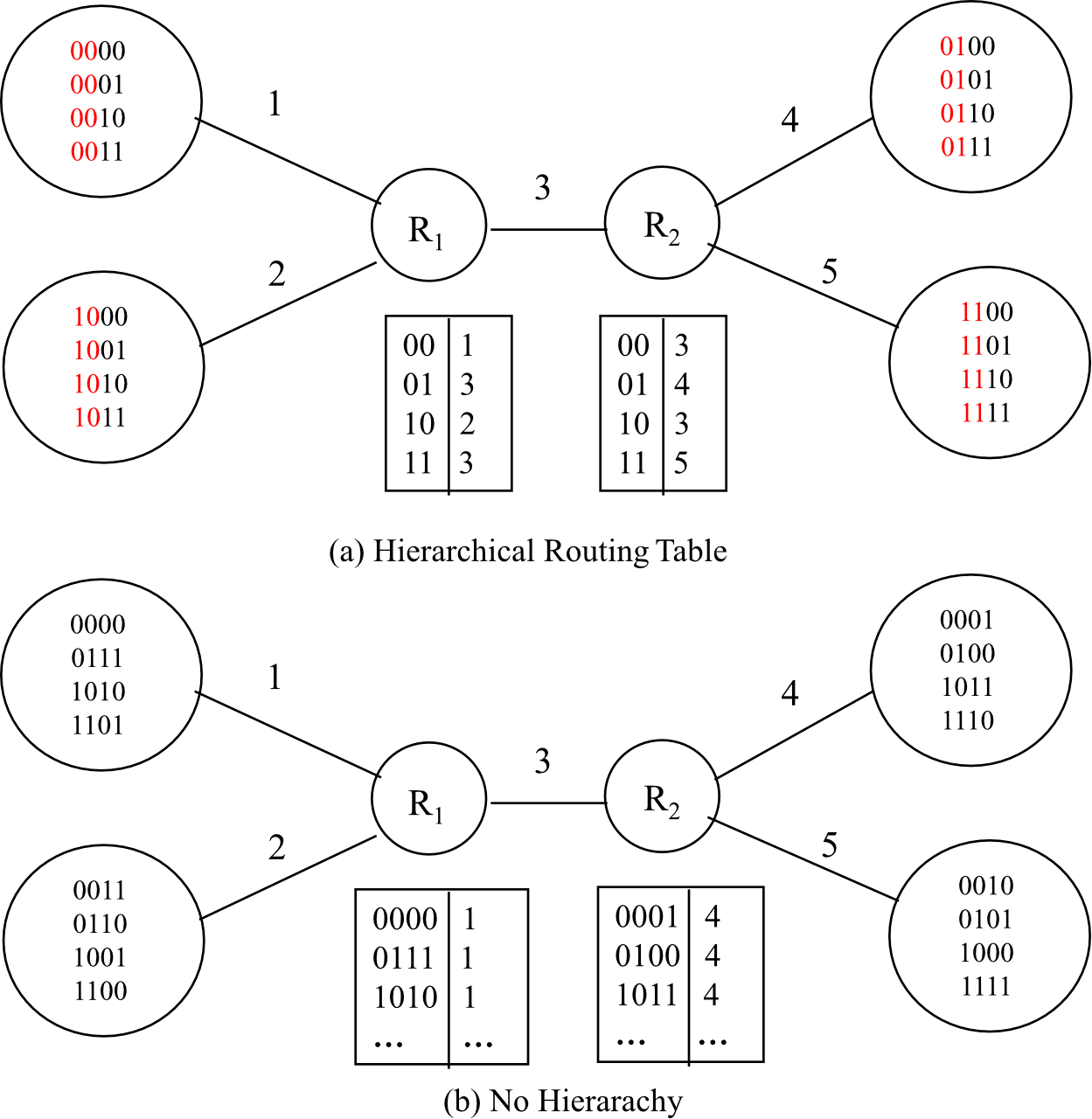
Analogy: Like postal addresses - mail is first routed to the city (network prefix), then to the street (subnet), then to the house number (host). You don't need every postman to know every house address in the country.
กระจายไปศูนย์ใหญ่ก่อน แล้วค่อยให้ใกล้ ๆ ที่รู้ส่งต่อไป เหมือน Zip Code
IP Hierarchical Addressing
Structure
Where:
Computing Routes Dynamically
กลับมาในส่วนของ Dynamic ที่ Router คำนวณหาเส้นทางเอง - การจะบอกได้ว่าเส้นทางไหนดีที่สุด ก็ต้องมีตัวชี้วัดถูกป้ะ นั่นก็คือ Cost นั่นเอง
Core Concepts
- Best path based on metrics: hops, delay, bandwidth (Cost อาจจะเป็นพวกนี้)
- Generally called cost
- Shortest path = path with minimum cost
Requirements
- Routing algorithm must be configured with metric to use
- Routers exchange routing information to obtain metric values for different links
Two Main Algorithm Types
- Distance Vector Routing
- Link State Routing
Algorithm นี้อยู่เบื้องหลัง Internet ทำงานเงียบ ๆ แต่ทำให้เราใช้งานได้อย่างราบรื่นเลยล่ะ
Importance
- Routing information exchange is the most critical network function
- Must be efficient and not consume excessive bandwidth
- Usually invisible to users but always running
Distance Vector Routing
Core Mechanism
หัวใจ = เรียนรู้จากเพื่อนบ้าน: Router แต่ละตัวจะดูแล/รักษา ข้อมูลชุดนึง เรียกว่า “Distance Vector” ซึ่งบอกว่า สำหรับฉัน การจะไปถึงปลายทาง (X,Y,Z) เนี่ยต้องใช้ Cost เท่าไหร่ แล้วต้องส่งผ่านเพื่อนบ้านคนไหน
หลังจากนั้นมันก็จะส่ง DV เนี่ยแหละ ให้เพื่อนบ้านของมัน เป็นระยะ ๆ แล้วอัปเดตเรื่อย อัปเดตใน DV ของตัวเอง
- Every router maintains its distance vector (DV)
- Records distance to each other host
- Routers exchange DV with neighbors periodically
- Upon receiving neighbor's DV:
- Check if better routes exist through that neighbor
- If yes, modify own DV
- Routing table derived directly from DV
Algorithm
- Uses Bellman-Ford Algorithm
- ถ้า Node เป็นจุดพักที่ดีที่สุดในเส้น A-B แล้ว เส้นทางจาก A-n-B ก็ต้องดีที่สุดด้วยเหมือนกัน
Link State Routing
หัวใจ = ทุกคนต้องรู้ข้อมูลจริงทั้งหมด: แทนที่จะเชื่อจากเพื่อนบ้าน วัดอะไรที่ต่อตรงกับตัวเองด้วยตัวเองเลย
- จากนั้นก็สร้าง Packet เล็ก ๆ: LSP ที่บรรจุข้อมูล Link ไว้ แล้วทำการกระจาย LSP นี้ออกไปให้ Router ในเครือข่ายได้รับรู้
- พอเพื่อน ๆ ได้รับ LSP ครบทุกตัวแล้ว แต่ละตัวก็จะเอาข้อมูล LSP เหล่านั้นมาประติดประต่อกัน สร้างเป็นแผนที่ฉบับสมบูรณ์ของเครือข่ายแบบสมบูรณ์เลยล่ะ (ทุกคนมีแผนที่เดียวกัน)
Core Mechanism
- Every router maintains Link State Packet (LSP)
- Records state information of links to all neighbors
- Router floods its LSP to entire network
- Sent to all routers
- Triggered whenever link state changes
- Upon receiving LSPs from other routers:
- Construct map of entire network
- Compute shortest paths using Dijkstra's algorithm
- พอทุกคนมีแผนที่แล้วก็เลือกทางที่ใกล้ที่สุดได้เลยล่ะ
- Derive routing table
Sample Network for Algorithm Examples
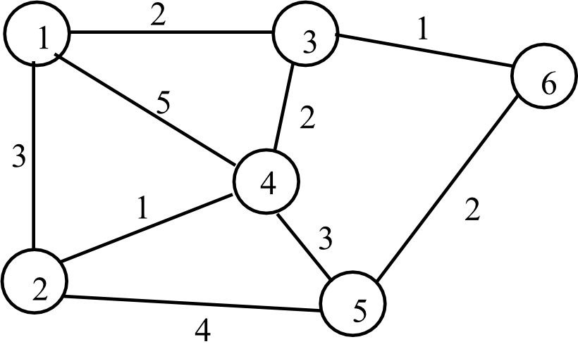
Network Structure
- 6 nodes (1-6)
- Edges represent links with associated costs
- Link costs shown as numbers on edges
Assumptions
- Non-directed links (bidirectional)
- If directed, cost can be assigned per direction
Bellman-Ford Algorithm
Principle
If node N is on the shortest path from A to B, then:
- Path from A to N is also the shortest path
- Path from N to B is also the shortest path
Formalization
Definitions:
- Node computing path to destination
- = current minimum cost estimate from node to destination
- (destination to itself)
- = link cost from node to node
- if and not directly connected
Core Formula:
Or equivalently:
Algorithm Steps
- Initialization:
- for all
- Updating:
- For each : , where is 's neighbor
- Iteration:
- Repeat step 2 until no changes occur
Example Calculation
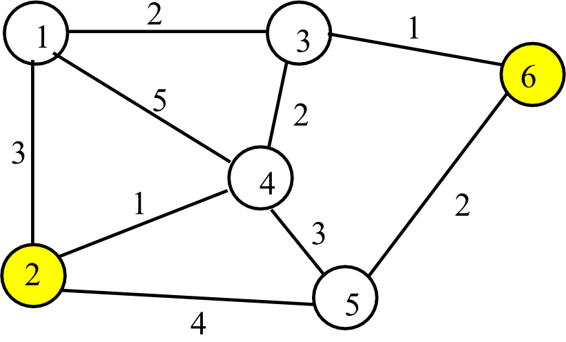
Computing shortest path from node 2 to node 6:
- If told: (cost from 1 → 6), and (cost from 2 → 1)
- Then 2 → 6 via 1 costs:
- If told: (cost from 4 → 6), and (cost from 2 → 4)
- Then 2 → 6 via 4 costs:
- If told: (cost from 5 → 6), and (cost from 2 → 5)
- Then 2 → 6 via 5 costs:
Result:
Shortest path from 2 → 6 goes through node 4.
Shortest Path Computation Example
Computing Paths to Node 6
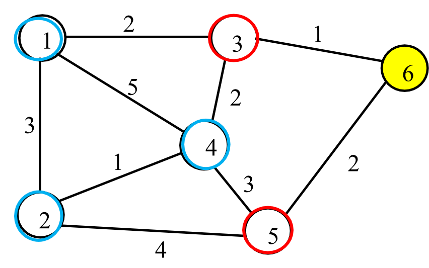
เริ่มจากติดจาก Node ปลายทางก่อน
Iteration Table:
| Iteration | Node 1 | Node 2 | Node 3 | Node 4 | Node 5 |
|---|---|---|---|---|---|
| Initial | (-1,∞) | (-1,∞) | (-1,∞) | (-1,∞) | (-1,∞) |
| 1 | (-1,∞) | (-1,∞) | (6,1) | (-1,∞) | (6,2) |
| 2 | (3,3) | (5,6) | (6,1) | (3,3) | (6,2) |
| 3 | (3,3) | (4,4) | (6,1) | (3,3) | (6,2) |
| 4 | (3,3) | (4,4) | (6,1) | (3,3) | (6,2) |
Notation: Each node labeled as where:
- = next node along current shortest path
- = current minimum cost from to destination
Result: Shortest path tree from all nodes to destination node 6 with edge costs of 2 hops for most paths.
Distance Vector and Routing Table
Example for Node 2
Distance Vector (full information): จะละเอียดว่า Routing Table ทั่วไปนะ
| Destination | Distance | Next Node |
|---|---|---|
| 1 | 3 | 1 |
| 3 | 3 | 4 |
| 4 | 1 | 4 |
| 5 | 4 | 5 |
| 6 | 4 | 4 |
Routing Table (used for forwarding):
| Destination | Next Node |
|---|---|
| 1 | 1 |
| 3 | 4 |
| 4 | 4 |
| 5 | 5 |
| 6 | 4 |
Analogy: The distance vector is like knowing both the total travel time and which highway to take for every destination. The routing table is the simplified version - just which highway to take.
How Node Computes Shortest Paths
Initial State at Node 2
| Destination | Distance | Next Node |
|---|---|---|
| 1 | 3 | 1 |
| 3 | ∞ | -1 |
| 4 | 1 | 4 |
| 5 | 4 | 5 |
| 6 | ∞ | -1 |
After Receiving Distance Vector from Node 4
Received from Node 4:
| Destination | Distance |
|---|---|
| 1 | 5 |
| 2 | 1 |
| 3 | 2 |
| 5 | 3 |
| 6 | ∞ |
Updated Distance Vector at Node 2:
| Destination | Distance | Next Node |
|---|---|---|
| 1 | 3 | 1 |
| 3 | 3 | 4 |
| 4 | 1 | 4 |
| 5 | 4 | 5 |
| 6 | ∞ | -1 |
(Node 2 learns about node 3 through node 4: )
After Receiving Distance Vector from Node 5
Received from Node 5:
| Destination | Distance |
|---|---|
| 1 | ∞ |
| 2 | 4 |
| 3 | ∞ |
| 4 | 3 |
| 6 | 2 |
Updated Distance Vector at Node 2:
| Destination | Distance | Next Node |
|---|---|---|
| 1 | 3 | 1 |
| 3 | 3 | 4 |
| 4 | 1 | 4 |
| 5 | 4 | 5 |
| 6 | 6 | 5 |
(Node 2 learns about node 6 through node 5: )
After Receiving Updated Distance Vector from Node 4
Received from Node 4 (updated):
| Destination | Distance |
|---|---|
| 1 | 5 |
| 2 | 1 |
| 3 | 2 |
| 5 | 3 |
| 6 | 3 |
Final Distance Vector at Node 2:
| Destination | Distance | Next Node |
|---|---|---|
| 1 | 3 | 1 |
| 3 | 3 | 4 |
| 4 | 1 | 4 |
| 5 | 4 | 5 |
| 6 | 4 | 4 |
(Node 2 finds better path to node 6 through node 4: )
Convergence achieved! ✓
Distributed Implementation of Bellman-Ford
Key Characteristics
- Fully distributed: Algorithm executes at every node
- Each node computes shortest paths to all other nodes independently
- Prerequisites: Neighbors must exchange distance vectors periodically
- Update mechanism:
- When receiving neighbor's distance vector
- Check for new shortest paths through that neighbor
- Modify own distance vector if better path found
- Mutual dependency:
- Nodes receive distance vectors from neighbors mutually
- Computations depend on each other (circular dependency)
- Eventually converges to correct results despite circular dependency
Broadcast Strategies
- Periodic updates: Regular scheduled broadcasts of distance vectors
- Triggered updates: Immediate broadcast when distance vector changes
Computing Formula
For each node :
Analogy: Like a group of friends sharing traffic updates - everyone tells their neighbors about road conditions, and eventually everyone learns the best routes, even though no one has the complete picture initially.
Link Failure Handling
Recomputation When Link Breaks
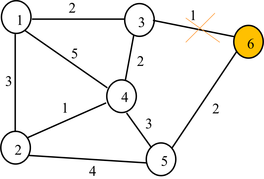
Routing Table at Node 6:
| Update | Node 1 | Node 2 | Node 3 | Node 4 | Node 5 |
|---|---|---|---|---|---|
| Before break | (3,3) | (3,4) | (3,1) | (3,3) | (5,2) |
| After break | (3,3) | (3,4) | (-1,∞) | (3,3) | (5,2) |
| 1 | (3,3) | (3,4) | (5,7) | (3,3) | (5,2) |
| 2 | (5,9) | (5,6) | (5,7) | (5,5) | (5,2) |
| 3 | (5,9) | (5,6) | (5,7) | (5,5) | (5,2) |
| 4 | (5,9) | (5,6) | (5,7) | (5,5) | (5,2) |
Notation: (next_node, distance)
Assumption: Computation and transmission are synchronized
Result: Eventually converges to new stable state
Counting to Infinity Problem
อันนี้เป็นปัญหาของ DV Table: ปัญหานี้จะเกิดขึ้นก็ต่อเมื่อ Link ขาด แล้ว Router มันกระจายข้อมูลไม่ทันไรงี้อะ Router ตัวก่อนหน้าก็ยังคิดว่า มาทางนี้โอเคอยู่ (หรืออาจจะทำให้เกิดการส่งข้อมูลวนไปมา) ค่า Cost ก็จะเพิ่มไปเรื่อย ๆ เลยล่ะ
The Problem
Scenario: Linear network 1-2-3-4, link between 3-4 breaks
Before break:
| Node | Node 1 | Node 2 | Node 3 |
|---|---|---|---|
| - | (2,3) | (3,2) | (4,1) |
After break:
| Update | Node 1 | Node 2 | Node 3 |
|---|---|---|---|
| After break | (2,3) | (3,2) | (2,3) |
| 1 | (2,3) | (3,4) | (2,3) |
| 2 | (2,5) | (3,4) | (2,5) |
| 3 | (2,5) | (3,6) | (2,5) |
| 4 | (2,7) | (3,6) | (2,7) |
| ... | ... | ... | ... |
Problem Characteristics
- Costs keep increasing indefinitely
- Eventually guess destination is unreachable when costs become very large
- Bad news travels slowly
- Good news travels quickly (if broken link restored, convergence is fast)
Analogy: Like a game of telephone where everyone keeps saying "I heard the store is further away than you said" and the distance keeps growing in everyone's minds, even though the store is actually closed.
Solution: Split Horizon with Poisoned Reverse
Technique การแก้ปัญหาสิ่งนี้
Technique
Idea:
- Split Horizon — อย่าบอกข้อมูลกลับไปในทางที่ได้รับมา ง่าย ๆ คือ ถ้า Router A รู้เส้นทางไป X (ผ่าน B), Router A ก็จะไม่ประกาศไปให้ B ทราบอีก เพราะ B ควรรู้อยู่แล้ว
- Poisoned Reverse — โกหก Router B ไปเลย ว่า Cost ที่ฉันจะไป X คือ นะ เพื่อให้ B รู้ว่า A มันต้องพึ่ง B นะ! จะไปพึ่ง A กลับไม่ได้แล้ว
Rule: Set minimum cost to destination as (poison) if:
- The neighbor is the next node along the shortest path
- Before sending out distance vector to that neighbor
Effect on Counting to Infinity
Same scenario with poisoned reverse:
| Update | Node 1 | Node 2 | Node 3 |
|---|---|---|---|
| Before break | (2,3) | (3,2) | (4,1) |
| After break | (2,3) | (3,2) | (-1,∞) |
| 1 | (2,3) | (-1,∞) | (-1,∞) |
| 2 | (-1,∞) | (-1,∞) | (-1,∞) |
Result: Quickly converges to correct state (unreachable) ✓
Analogy: Like telling your friend "don't ask me about the route to the store, you're the one who told me about it" - prevents circular dependency.
Dijkstra's Algorithm & Link State Routing
Dijkstra's Algorithm Overview
Given: Complete network topology (graph)
Goal: Find shortest paths from node to all other nodes
Process:
- Find closest neighbor node from node → Modify costs
- Find second closest node from (neighbor of or ) → Modify costs
- Find third closest node from (neighbor of , , or ) → Modify costs
- Continue until all nodes processed...
How Nodes Obtain Network Topology
Link State Packet (LSP):
- Records node's neighbors and costs to them
- Every node creates its own LSP
Flooding Mechanism:
- Every node floods its LSP to entire network (all nodes)
- Triggered at initialization or when link status changes
Topology Construction:
- Node receives all LSPs from all other nodes
- Constructs complete network map
- Applies Dijkstra's algorithm to compute shortest paths
- Derives routing table
Dijkstra's Algorithm Example
Computation from Node 1
Iteration Table:
| Iteration | N | D₂ | D₃ | D₄ | D₅ | D₆ |
|---|---|---|---|---|---|---|
| Initial | {1} | 3 | 2 | 5 | ∞ | ∞ |
| 1 | {1,3} | 3 | 2 | 4 | ∞ | 3 |
| 2 | {1,2,3} | 3 | 2 | 4 | 7 | 3 |
| 3 | {1,2,3,6} | 3 | 2 | 4 | 5 | 3 |
| 4 | {1,2,3,4,6} | 3 | 2 | 4 | 5 | 3 |
| 5 | {1,2,3,4,5,6} | 3 | 2 | 4 | 5 | 3 |
Where:
- = set of nodes for which shortest path is known
- = current shortest distance to node
Resulting Shortest Path Tree
From Node 1:
- 1 → 2 (cost 3)
- 1 → 3 (cost 2)
- 1 → 3 → 4 (cost 4)
- 1 → 3 → 5 (cost 5)
- 1 → 3 → 6 (cost 3)
Routing Table for Node 1
| Destination | Next Node | Cost |
|---|---|---|
| 2 | 2 | 3 |
| 3 | 3 | 2 |
| 4 | 3 | 4 |
| 5 | 3 | 5 |
| 6 | 3 | 3 |
Link State Packets (LSP) Example
LSP for 6-Node Network
- LSP₁: (2,3), (3,2), (4,5)
- LSP₂: (1,3), (4,1), (5,4)
- LSP₃: (1,2), (4,2), (6,1)
- LSP₄: (1,5), (2,1), (5,3), (3,2)
- LSP₅: (2,4), (4,3), (6,2)
- LSP₆: (3,1), (5,2)
Format: (neighbor_node, cost)
Purpose:
- LSP records current neighbors and corresponding costs
- From all LSPs, any node can construct complete network map
Comparison: Distance Vector vs. Link State Routing
Distance Vector Routing
Characteristics:
- ✓ Distance vector records costs to all nodes
- ✓ Neighbors exchange distance vectors periodically
- ✗ Convergence occurs eventually and slowly
- ✗ Packets may loop temporarily during convergence
- ✗ Reacts to link failure very slowly
- ✗ Counting-to-infinity problem
Best for: Smaller, stable networks (เหมาะกับเครือข่ายขนาดเล็ก ไม่ซับซ้อน ไม่ค่อยเปลี่ยนแปลง)
Link State Routing
Characteristics:
- ✓ LSP records costs to neighbors only
- ✓ Flood LSP to ==entire network== when topology changes
- ✓ Reacts to network failure fast
- ✗ Excessive flooding when topology changes frequently
- ✗ Consumes network bandwidth during updates
Best for: Larger, dynamic networks (เครือข่ายขนาดใหญ่ ซับซ้อน ต้องการปรับตัวเร็ว)
Common Feature
Distributed routing: Route from source to destination is distributed and synthesized by all nodes along the path
Analogy:
- Distance Vector = Everyone shares their entire address book with neighbors, updates spread slowly like gossip, เชื่อเพื่อนบอกต่อ ช้าหน่อย
- Link State = Everyone shouts their immediate connections to everyone, updates spread fast like broadcasting news, ขอข้อมูลดิบ มาคิดเองดีกว่า แม่นกว่า แต่ก็ใช้ทรัพยากรเยอะกว่า
Summary
Key Takeaways
- Routing determines best paths in networks based on various metrics (hops, delay, bandwidth)
- Two main dynamic routing protocols:
- Distance Vector (Bellman-Ford): Simple, slow convergence, prone to loops
- Link State (Dijkstra): Complex, fast convergence, higher bandwidth usage
- Important concepts:
- Routing tables store forwarding information
- Hierarchical addressing reduces table size
- Virtual circuits use local VCIs for efficiency
- Split horizon prevents counting-to-infinity problem
- Trade-offs exist between:
- Simplicity vs. performance
- Convergence speed vs. bandwidth usage
- Centralized vs. distributed control