Chapter 12 - Convolutional Neural Networks

A type of neural network that is suitable for handling multidimensional data, e.g. image, video.

12.1 Neural Networks and Images

Problems with Flattening Images

When an image is flattened into a vector before feeding it into a neural network with fully connected layers, several problems arise:

ถ้าจะใช้เอาไปใช้แบบปกติต้อง Flatten image ให้กลายเป็น Vector ก่อน (Because Neural Network require data to be a vector)

1. Adjacency of Pixels is Not Taken Into Account

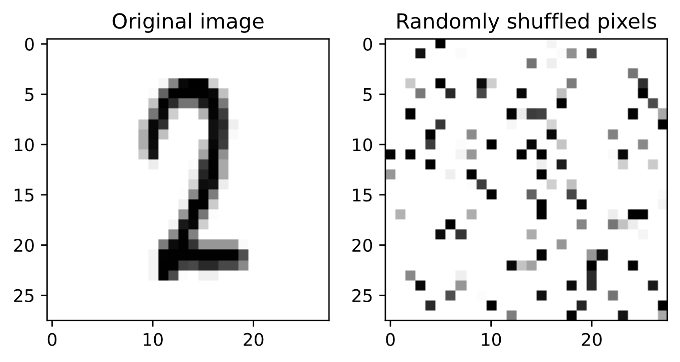
• Training the network with either the original image or the image with randomly shuffled pixels would yield the same result
• The spatial relationship between pixels is completely lost
• Adjacent pixels that might represent the same object or pattern are treated as independent features

Analogy: Imagine reading a book where all the letters are randomly shuffled. Even though all the letters are still there, you can't understand the meaning because the order (adjacency) matters. Similarly, pixel positions in images carry crucial information.

2. The Same Pattern Occurring in Different Locations May Not Be Recognized

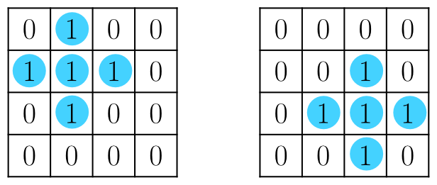
• Weights are not shared across locations
• A pattern learned at one position won't be recognized at another position
• The network would need to learn the same pattern multiple times for different locations

Analogy: If you learn to recognize a cat in the top-left corner of an image, you should be able to recognize it anywhere else. But with fully connected layers, it's like having to relearn what a cat looks like for every possible position in the image.

3. High-Resolution Images Require Very Large Numbers of Weights

• An image with $n$ pixels connected to a layer with $n$ units requires:
  $\boxed{\underbrace{\frac{(n)(n)}{2}}_{\vec{W}} + \underbrace{\frac{n}{2}}_{\vec{b}} \text{ parameters}}$
• This leads to computational inefficiency and increased risk of overfitting

Analogy: If you wanted to personally shake hands with every person in a stadium (fully connected), you'd need millions of handshakes. But if you just wave to everyone (shared weights), one gesture reaches everyone.

12.2 Convolution Operations

จะจัดการปัญหาเหล่านั้นได้ยังไง ก็มีไอเดีย Convolution Operations ขึ้นมาใช้ใน Neural Network

Mathematical Definition

Convolution is defined as an operation between two functions:

$\boxed{[f \ast g](t) = \int_{-\infty}^{+\infty} f(\tau)g(t - \tau)d\tau}$

• This is the integral of the product of $f$ and $g$ after $g$ is flipped and shifted

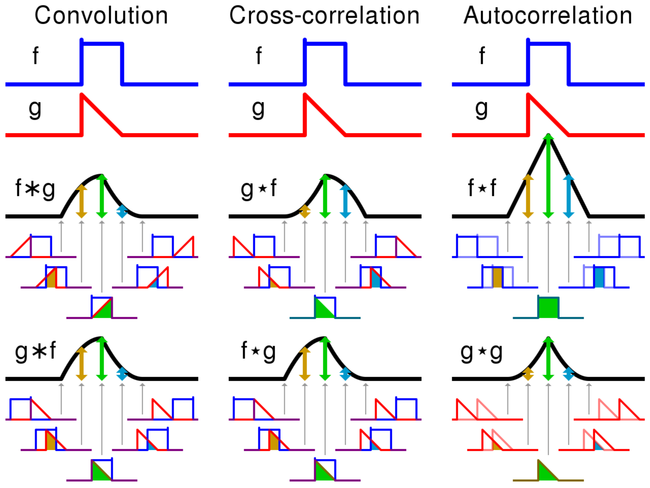
• The convolution operation is similar to cross-correlation when neither $f$ nor $g$ is flipped

Analogy: Think of convolution as sliding a template over a signal and measuring how well they match at each position. The flipping is like reading the template backwards as you slide it.

12.2.1 Cross-Correlation Operations

1D Cross-Correlation

Given an input vector $\boldsymbol{x}$ and a vector kernel $\boldsymbol{k}$ of size $l$, the cross-correlation operation $\boldsymbol{x} \star \boldsymbol{k}$ is defined as:
$\boxed{(\boldsymbol{x} \star \boldsymbol{k})_i = \sum_{u=0}^{l-1} k_{u+1}x_{i+u}}$
For example, when $l = 3$:
$(\boldsymbol{x} \star \boldsymbol{k})_i = \sum_{u=0}^{2} k_{u+1}x_{i+u} = k_1x_i + k_2x_{i+1} + k_3x_{i+2}$

Key Point: The output at position $i$ is the dot product between the kernel $\boldsymbol{k}$ and a portion of $\boldsymbol{x}$ of size $l$ starting from $x_i$.

Analogy: Imagine you have a magnifying glass (the kernel) that you slide over a line of text (the input). At each position, you multiply what you see through the glass by some weights and sum them up to get a single number.

Example 12.1

Let $\boldsymbol{x} = \Big[1\ 4\ 2\ 0\ 9\ 1\ 3\Big]$ and $\boldsymbol{k} = \begin{bmatrix} \frac{1}{4} \\ \frac{2}{4} \\ \frac{1}{4} \end{bmatrix}$

Calculate $\boldsymbol{z} = \boldsymbol{x} \star \boldsymbol{k}$:

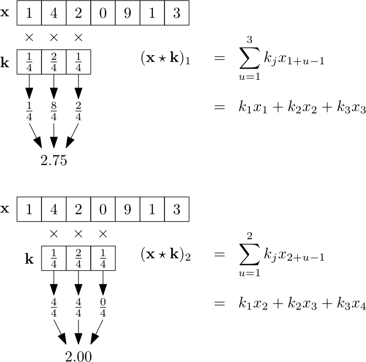
Position 1:
$(\boldsymbol{x} \star \boldsymbol{k})_1 = k_1x_1 + k_2x_2 + k_3x_3 = \frac{1}{4}(1) + \frac{2}{4}(4) + \frac{1}{4}(2) = 2.75$

Position 2:
$(\boldsymbol{x} \star \boldsymbol{k})_2 = k_1x_2 + k_2x_3 + k_3x_4 = \frac{1}{4}(4) + \frac{2}{4}(2) + \frac{1}{4}(0) = 2.00$
And so on.

• $\vec{\boldsymbol{z}}=\Big[2.75, 2.00, \dotso\Big]$

2D Cross-Correlation

The cross-correlation operation can be applied to 2D arrays:

$\boxed{(\boldsymbol{x} \star \boldsymbol{k})_{i,j} = \sum_{u=0}^{k_h-1} \sum_{v=0}^{k_w-1} k_{u+1,v+1}x_{i+u,j+v}}$

where a kernel $\boldsymbol{k}$ is a 2D array with size $k_h \times k_w$.

Example 12.2

When $\boldsymbol{k} = \begin{bmatrix} k_{1,1} & k_{1,2} \\ k_{2,1} & k_{2,2} \end{bmatrix}$:

$(\boldsymbol{x} \star \boldsymbol{k})_{i,j} = k_{1,1}x_{i,j} + k_{1,2}x_{i,j+1} + k_{2,1}x_{i+1,j} + k_{2,2}x_{i+1,j+1}$

Example 12.3

Conduct a cross-correlation operation:

$\begin{bmatrix} 1 & 4 & 1 & 1 & 2 \\ 4 & 3 & 1 & 2 & 1 \\ 5 & 2 & 2 & 2 & 5 \\ 1 & 3 & 2 & 4 & 3 \end{bmatrix} \star \begin{bmatrix} -1 & -1 & -1 \\ -1 & 8 & -1 \\ -1 & -1 & -1 \end{bmatrix} = \begin{bmatrix} 4 & -9 & 1 \\ -5 & -3 & -4 \end{bmatrix}$

Calculation for position (1,1):
$(\boldsymbol{x} \star \boldsymbol{k})_{1,1} = (-1)(1) + (-1)(4) + (-1)(1) + (-1)(4) + (8)(3) + (-1)(1) + (-1)(5) + (-1)(2) + (-1)(2) = 4$

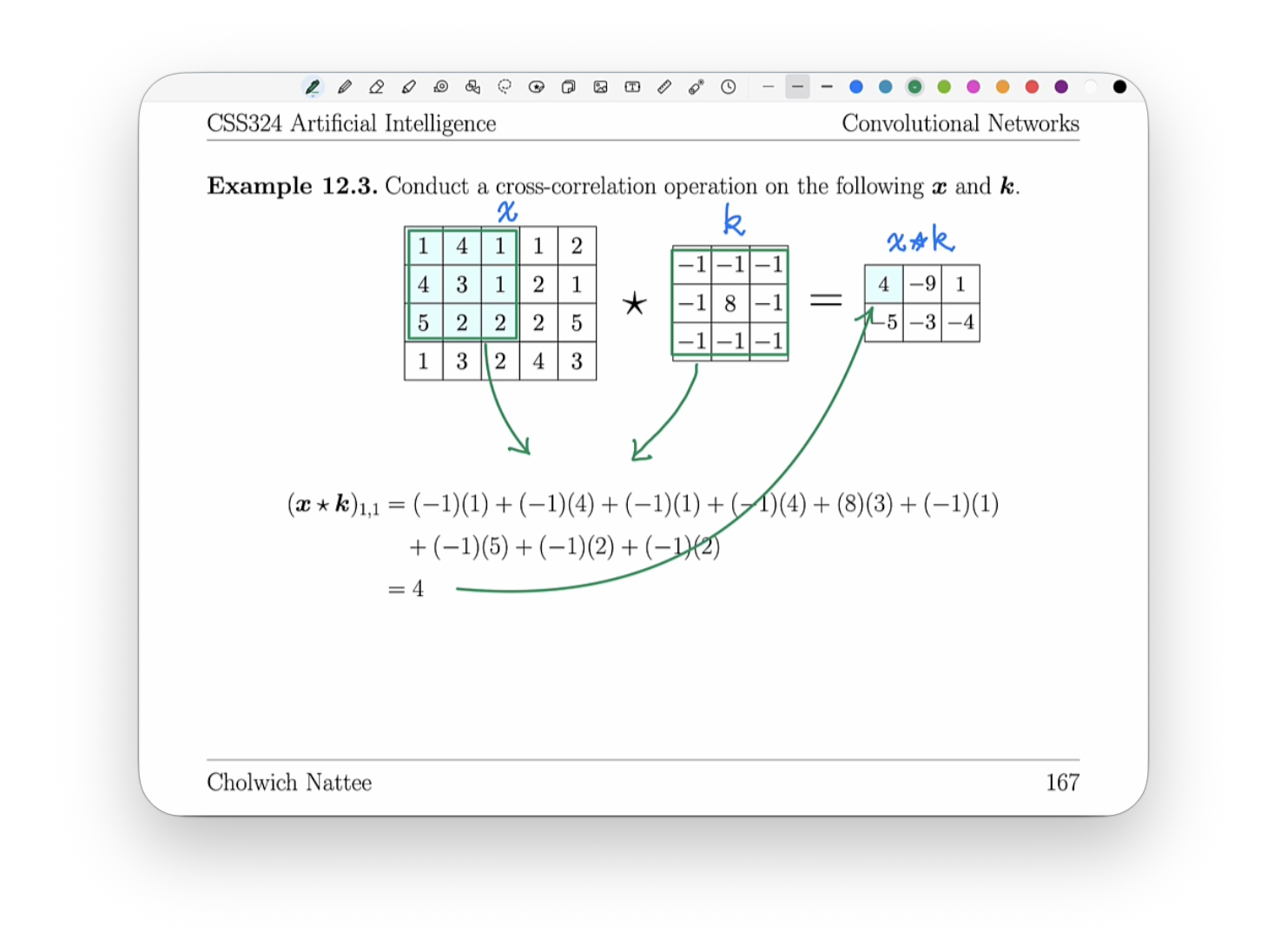
Analogy: This is like using a stamp on paper. You press the stamp (kernel) at different positions on the paper (input image), and each press creates a mark (output value) based on how the stamp pattern aligns with what's underneath.

12.2.2 Boundary Conditions

อันนี้โชว์เลยว่า สมมติรู้ Dimension ของ Matrix A ซึ่งจะ $\star$ Matrix B เป็นสูตรบอกว่า Dimension C เป็นเท่าไหร่

Valid Convolution/Cross-Correlation

• Given a 2D array $\boldsymbol{x}$ with $n_h$ rows and $n_w$ columns
• Given a kernel $\boldsymbol{k}$ with $k_h$ rows and $k_w$ columns
• The convolution operation $\boldsymbol{x} \star \boldsymbol{k}$ returns a 2D array with shape:

$\boxed{\underbrace{(n_h - k_h + 1)}_{\text{\#rows}} \times \underbrace{(n_w - k_w + 1)}_{\text{\#cols}}}$

Same Convolution/Cross-Correlation

• To output an array of the same size as the input, pad the input array with zeros
  • We want this!!
• The number of padded zeros $p$ is given by the kernel size $l$:

$\boxed{p = l - 1}$

Notation:

• $\star_v$ denotes valid convolution/cross-correlation
• $\star_s$ denotes same convolution/cross-correlation

Example

Given:

Compute padding:

Split evenly:

After zero-padding:

Now the output shape after convolution with a $3 \times 3$ kernel is:

Analogy: Valid convolution is like scanning a document with a scanner that must stay completely on the page - you lose the edges. Same convolution is like extending the page with blank margins so the scanner can cover the original page completely.

Example 12.4

Conduct the same cross-correlation using $\boldsymbol{x}$ and $\boldsymbol{k}$ from the previous example.

For a $3 \times 3$ kernel:

• $p_h = 3 - 1 = 2$
• $p_w = 3 - 1 = 2$

$\text{Output size}=(6-3+1)\times(7-3+1)=4\times 5$
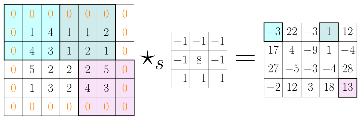
The input is padded with 2 rows/columns of zeros on each side, resulting in an output of the same size as the original input.

12.2.3 Strides

• By default, the kernel is slid to the right and down one element at a time
• Stride specifies the number of rows and columns moved per slide
• When the stride is $s_h \times s_w$, the output array shape for same cross-correlation is:
  • คราวนี้อยากเลื่อนทีละหลาย ๆ ช่องแล้ว ก็สามารถ Specify ได้

$\boxed{\left\lfloor \frac{n_h - k_h + p_h + s_h}{s_h} \right\rfloor \times \left\lfloor \frac{n_w - k_w + p_w + s_w}{s_w} \right\rfloor}$

Analogy: A stride is like skipping steps when walking. Stride 1 means taking every step, stride 2 means taking every other step. Larger strides cover the distance faster but with less detail.

Example 12.5

Same cross-correlation with stride $2 \times 2$:

The shape of the output is:
$\left\lfloor \frac{4 - 3 + 2 + 2}{2} \right\rfloor \times \left\lfloor \frac{5 - 3 + 2 + 2}{2} \right\rfloor = 2 \times 3$

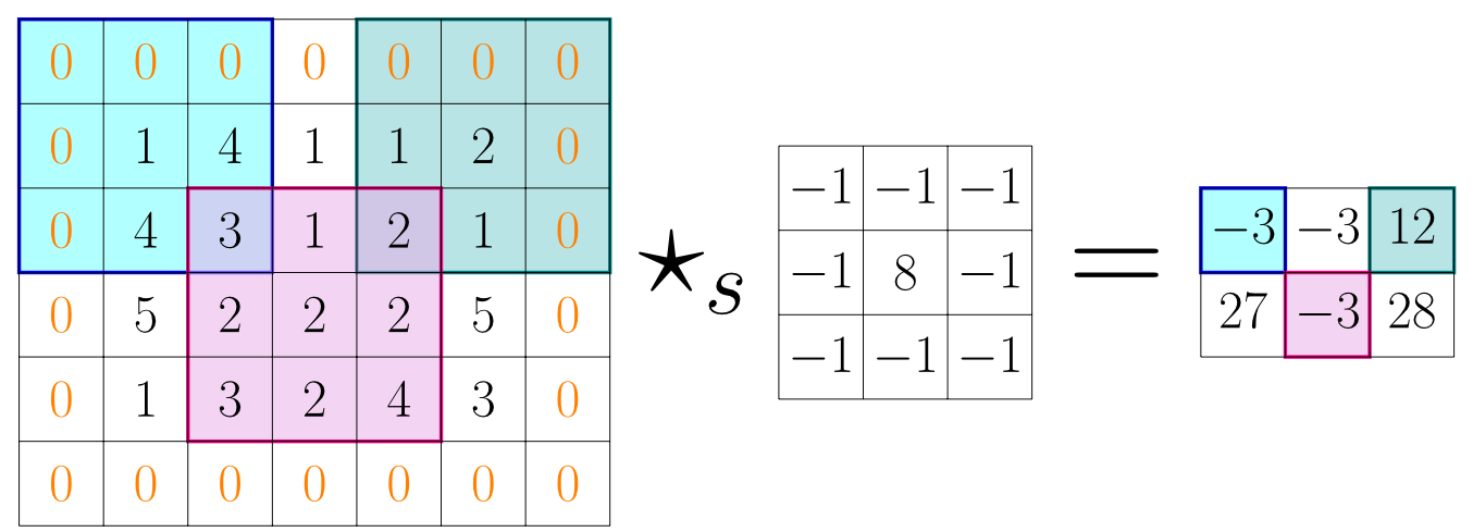
อันนี้ก็เลื่อนทีละ 2 เลย,
Formula ตอน Calculate ใช้ Original Matrix ไม่เอาที่ Pad แล้วนะ

12.2.4 Applications of Convolution/Cross-Correlation

In image processing, convolution operations are applied to process images:

• Various types of kernels have been designed to blur, sharpen, or detect edges of images

Example 12.6: Edge Detection

When $\boldsymbol{x}$ is an image and $\boldsymbol{k} = \begin{bmatrix} -1 & -1 & -1 \\ -1 & 8 & -1 \\ -1 & -1 & -1 \end{bmatrix}$:

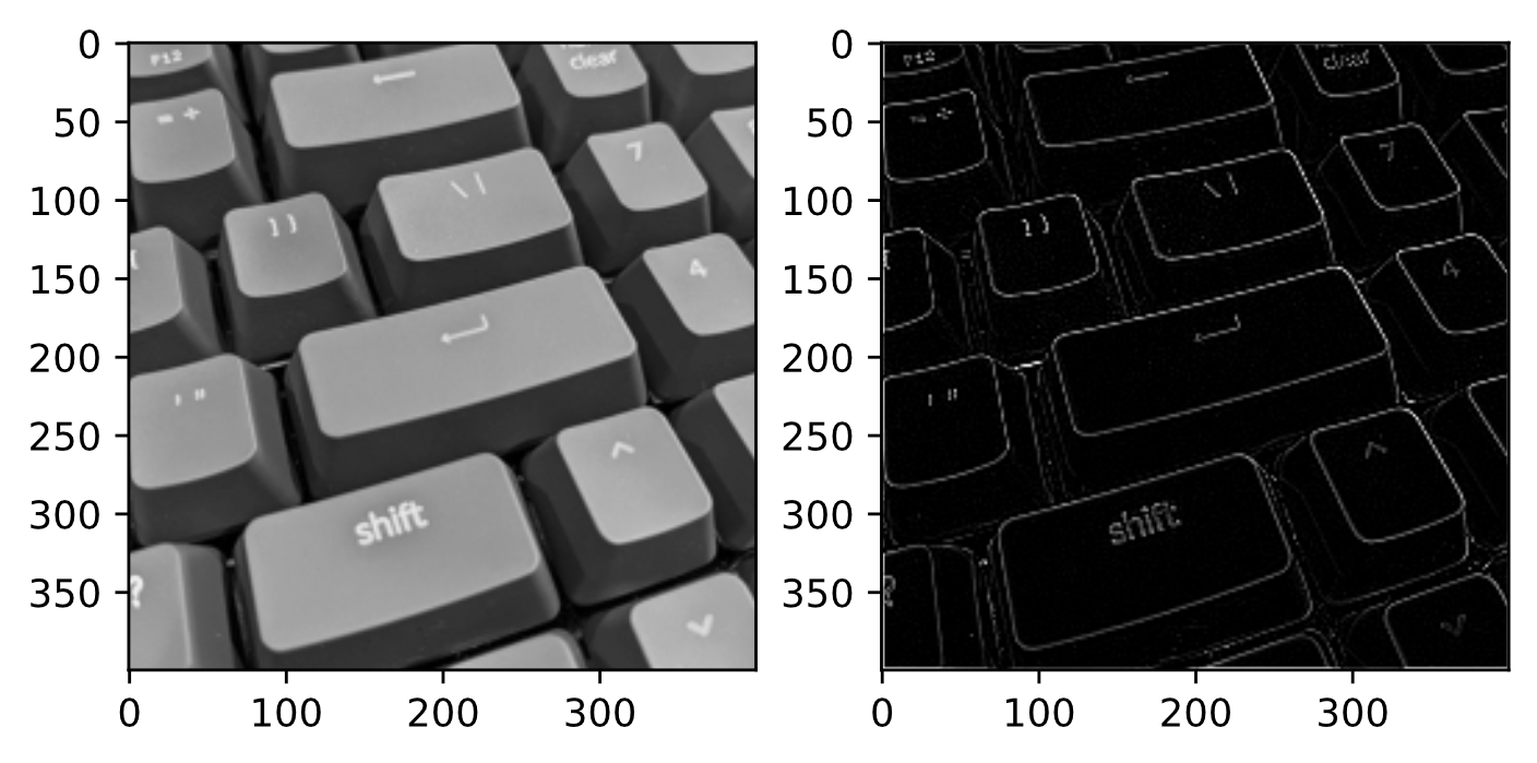
รูปซ้ายคือแค่ $\boldsymbol{x}$ แต่ขวาคือ Apply $\boldsymbol{k}$ ไปแล้ว ($\boldsymbol{x}\star\boldsymbol{k}$)

• The convolution of $\boldsymbol{x}$ and $\boldsymbol{k}$ detects edges in the image
• This kernel highlights regions where pixel values change rapidly

Key Insight: With a proper kernel, the convolution/cross-correlation operations can be used to extract features from local areas of input arrays.

Analogy: Different kernels are like different Instagram filters. An edge detection kernel is like a "sketch" filter that outlines objects, while a blur kernel is like a "soft focus" filter that smooths everything out.

12.3 Convolutional Neural Networks

A Convolutional Neural Network (CNN), introduced by LeCun et al. in 1998, is a neural network with convolutional layers containing filters (kernels) applied to the input array.

• Gradient descent optimizes kernel values
• Enables the network to extract meaningful features from local regions of the input

Analogy: CNNs are like having multiple adjustable filters on a camera. Instead of manually designing filters, the network learns which filters are best for the task through training.

12.3.1 Convolutional Layer

A convolutional layer is defined by:
$\boxed{\boldsymbol{z} = g((\boldsymbol{x} \star \boldsymbol{k}) + b\boldsymbol{J}_{h,w})}$
where:

• The shape of the output of the cross-correlation is $h \times w$
• $\boldsymbol{J}_{h,w}$ is an all-ones matrix with $h$ rows and $w$ columns
• $g$ is the activation function
• $b$ is the bias term

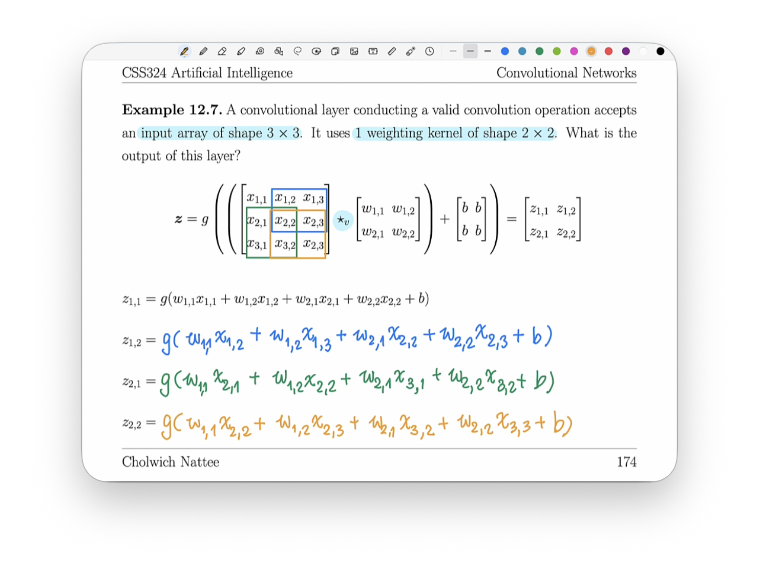
Example 12.7

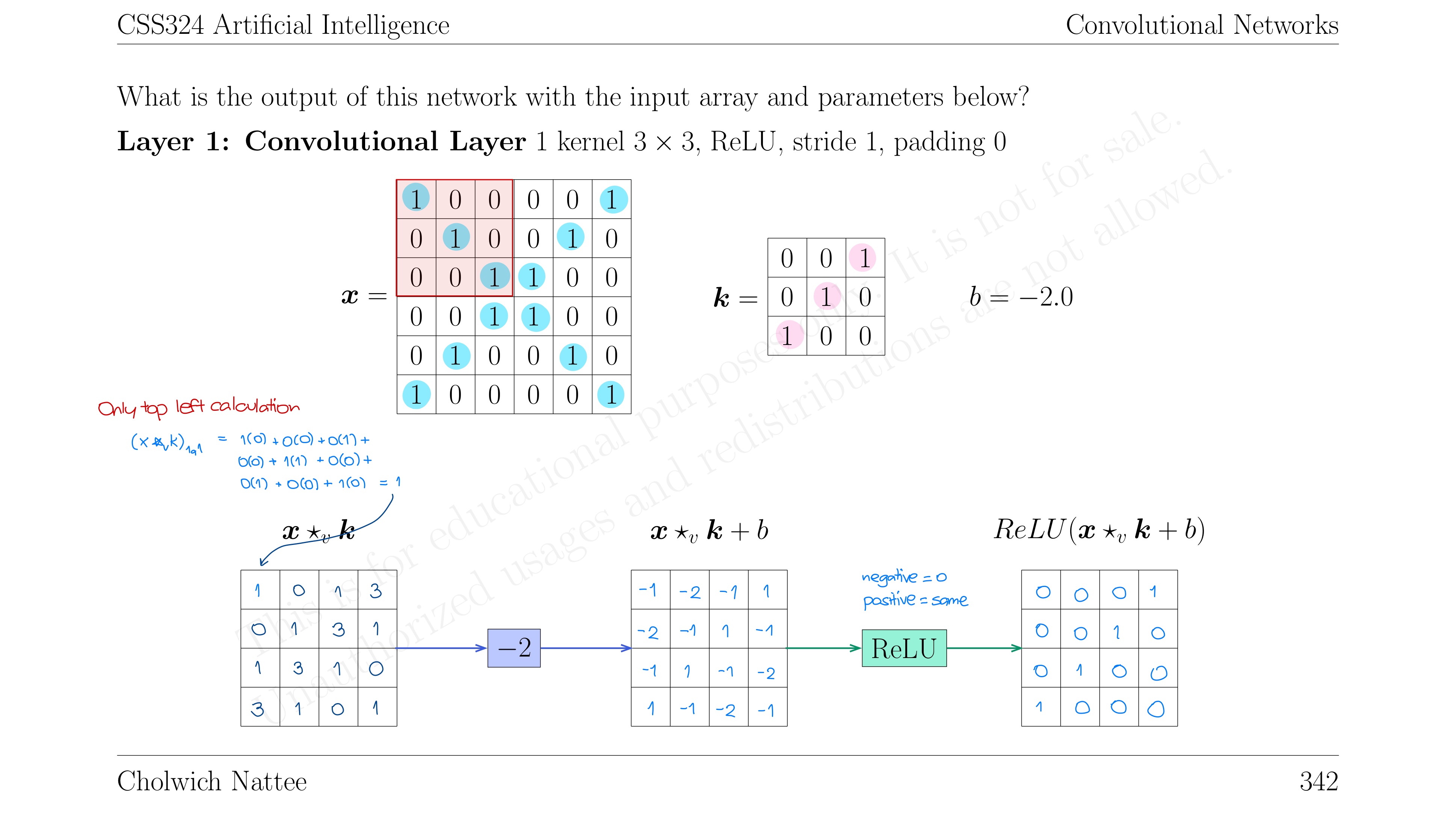
A convolutional layer conducting a valid convolution:

• Input array: $3 \times 3$
• 1 weighting kernel: $2 \times 2$
• Uses ReLU activation

Output calculation:

$\boldsymbol{z} = g\left(\begin{bmatrix} x_{1,1} & x_{1,2} & x_{1,3} \\ x_{2,1} & x_{2,2} & x_{2,3} \\ x_{3,1} & x_{3,2} & x_{3,3} \end{bmatrix} \star_v \begin{bmatrix} w_{1,1} & w_{1,2} \\ w_{2,1} & w_{2,2} \end{bmatrix} + \begin{bmatrix} b & b \\ b & b \end{bmatrix}\right) = \begin{bmatrix} z_{1,1} & z_{1,2} \\ z_{2,1} & z_{2,2} \end{bmatrix}$

where:

• $z_{1,1} = g(w_{1,1}x_{1,1} + w_{1,2}x_{1,2} + w_{2,1}x_{2,1} + w_{2,2}x_{2,2} + b)$
• $z_{1,2} = g(w_{1,1}x_{1,2} + w_{1,2}x_{1,3} + w_{2,1}x_{2,2} + w_{2,2}x_{2,3} + b)$
• $z_{2,1} = g(w_{1,1}x_{2,1} + w_{1,2}x_{2,2} + w_{2,1}x_{3,1} + w_{2,2}x_{3,2} + b)$
• $z_{2,2} = g(w_{1,1}x_{2,2} + w_{1,2}x_{2,3} + w_{2,1}x_{3,2} + w_{2,2}x_{3,3} + b)$

12.3.2 Receptive Field

Receptive field of a neuron refers to the part of the input that influences its output.

Growth of Receptive Field:

First hidden layer:

• Receptive field is the same size as the kernel

Deeper layers:

• The receptive field grows larger

With stride 1:

• Receptive field grows linearly
• In the $m$-th layer, size is: $\boxed{(l - 1)m + 1}$ where $l$ is the kernel size

With stride > 1:

• Receptive field grows exponentially
• Size in $m$-th layer: $\boxed{O(ls^m)}$ where $s$ is the stride

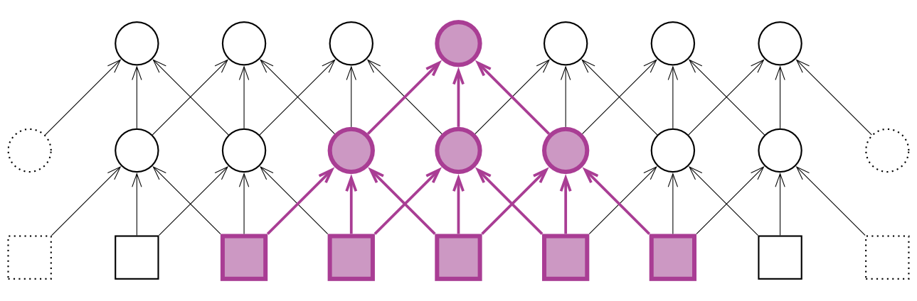
Analogy: The receptive field is like your field of vision. In the first layer, you see a small patch. In deeper layers, you see a larger area, like zooming out on a map. Each deeper layer combines information from a wider area of the original input.

12.3.3 Pooling Layer

A pooling layer extends the receptive field without trainable parameters.

Types of Pooling:

Average Pooling:

• Finds the average value within a moving window
• Works exactly like conducting a convolution operation with a uniform kernel array

Max Pooling:

• Finds the maximum value within a moving window
• Works as a kind of logical disjunction (OR operation)
• Most commonly used in modern CNNs

Analogy: Pooling is like summarizing information. If you have a paragraph, average pooling is like finding the average sentiment, while max pooling is like extracting the most important point. Max pooling says "if any strong feature is detected in this region, report it."

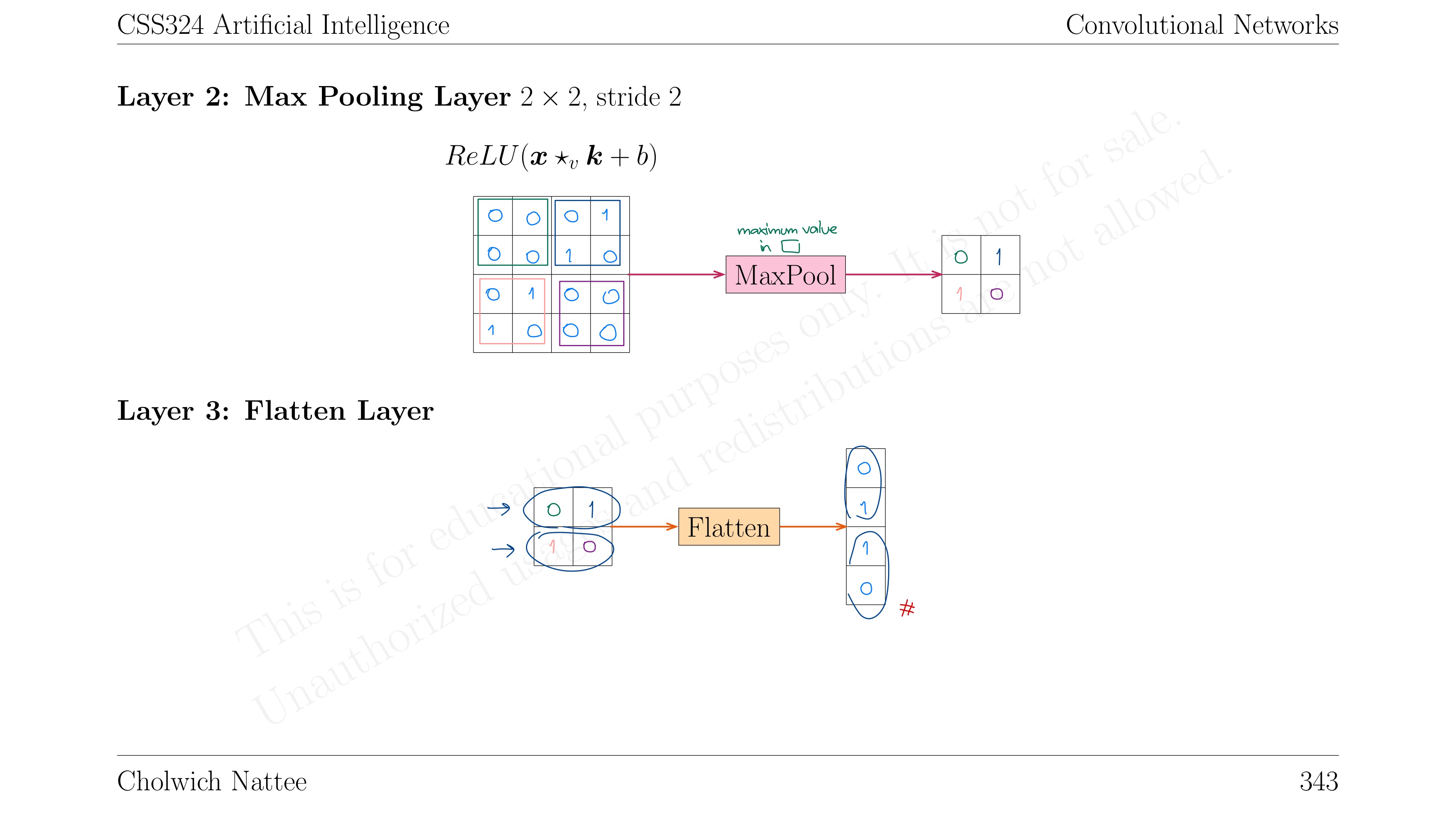
Example 12.8

Max pooling with window $2 \times 2$ and stride $1 \times 2$:

อันนี้แค่ Find maximum แต่ละช่องจากซ้ายมือ

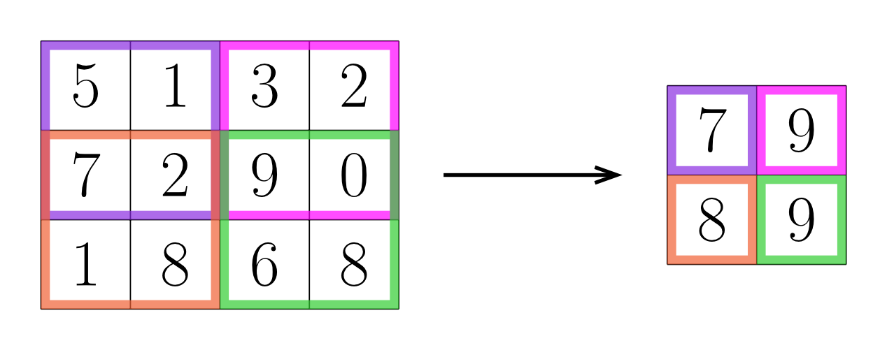
Input:
$\begin{bmatrix} 5 & 1 & 3 & 2 \\ 7 & 2 & 9 & 0 \\ 1 & 8 & 6 & 8 \end{bmatrix}$

Output:
$\begin{bmatrix} 7 & 9 \\ 8 & 9 \end{bmatrix}$

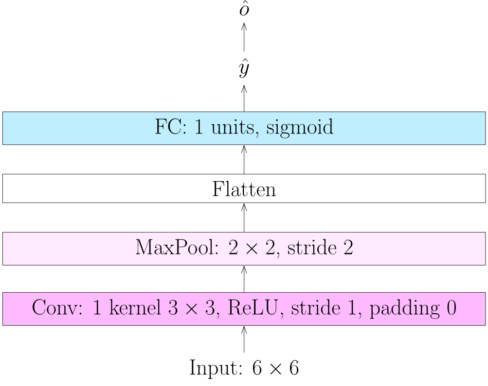
Example 12.9

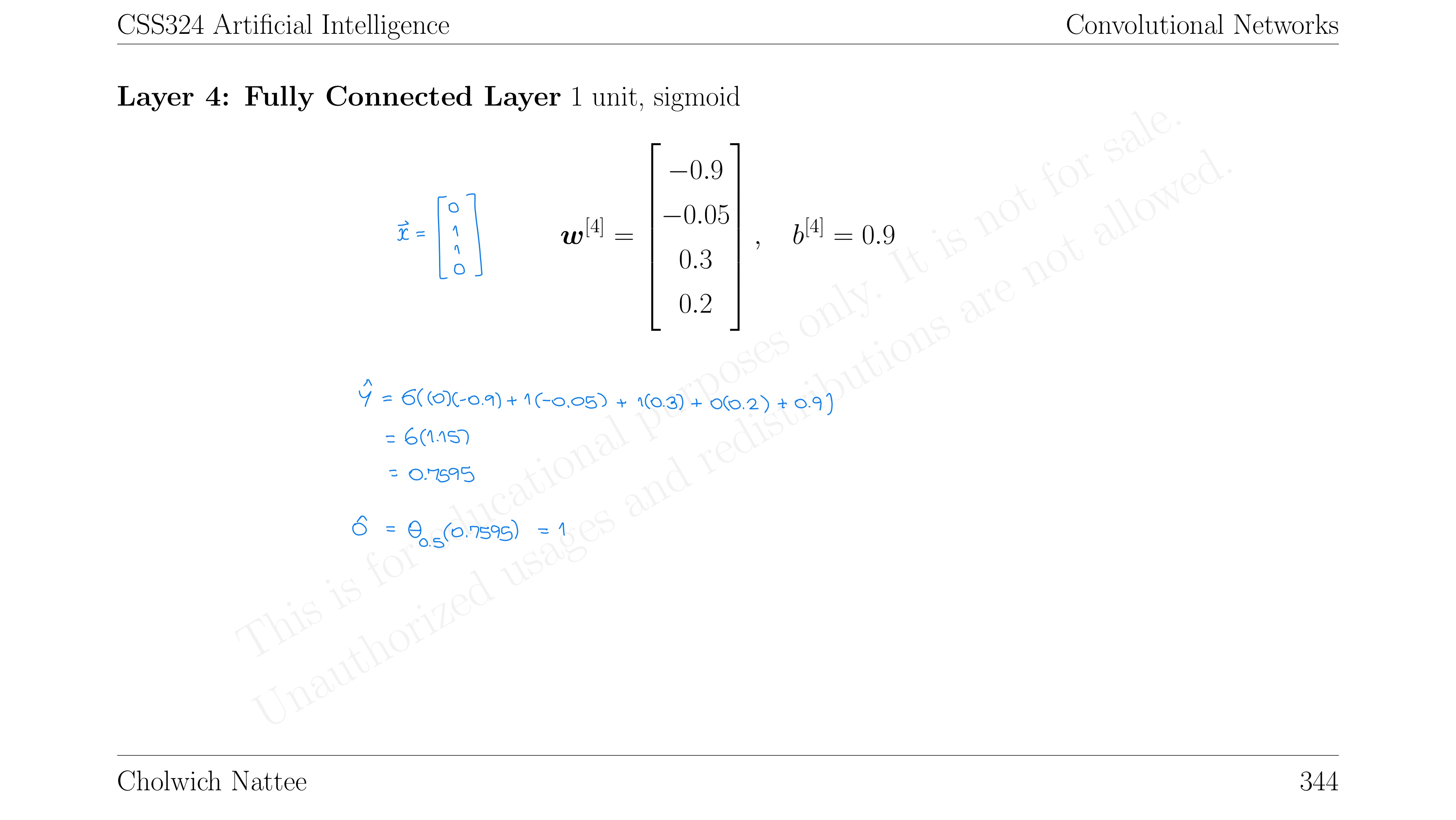
Given a CNN as shown below, calculate the output of the network when an input array of shape $6 \times 6$ is fed as input.

12.3.4 Multiple Input Channels

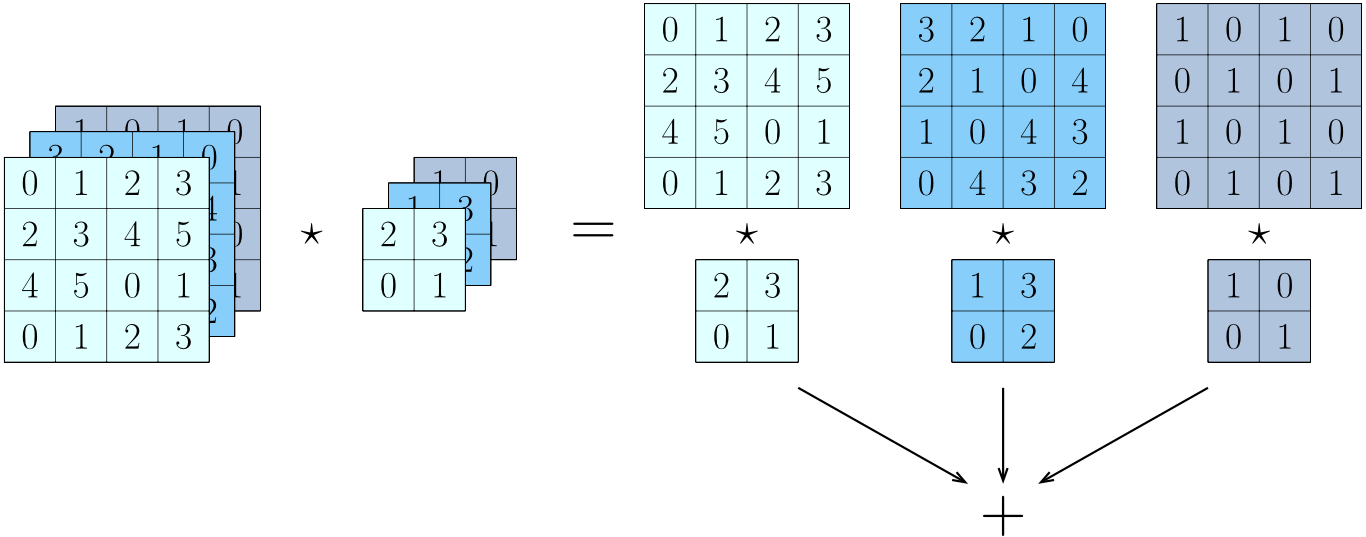
When input arrays contain multiple channels (e.g., RGB images with shape $h \times w \times c$ (#channels) where $c > 1$):

Process:

1. A kernel of shape $k_h \times k_w$ is created for each channel
2. The cross-correlation operation is performed for each channel
3. Results are summed together

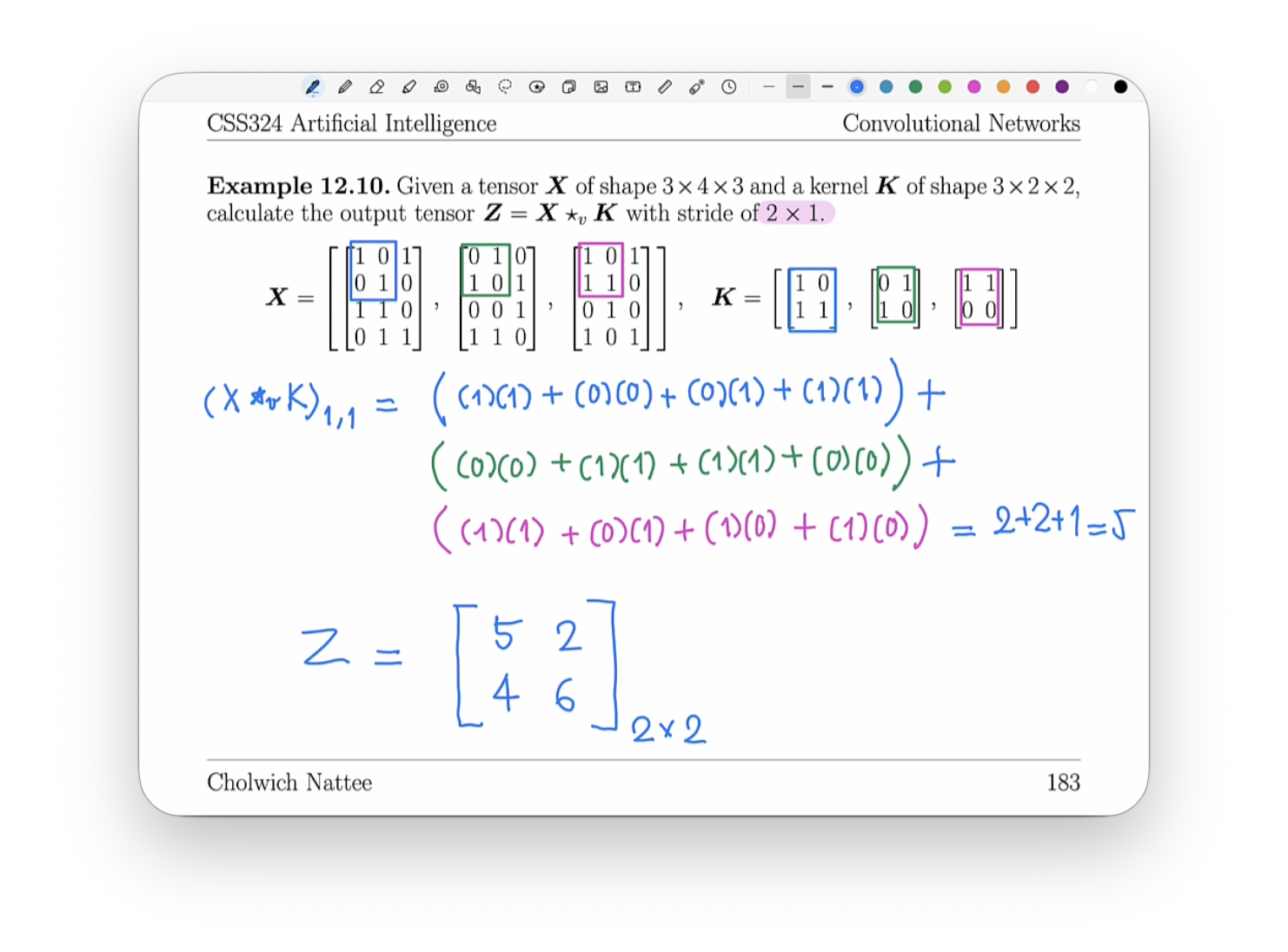
Example 12.10

Given:

• Tensor $\boldsymbol{X}$ of shape $3 \times 4 \times 3$ (3 channels)
• Kernel $\boldsymbol{K}$ of shape $3 \times 2 \times 2$ (one $2 \times 2$ kernel per channel)
• Stride of $2 \times 1$

The operation:

1. Apply each of the 3 kernels to its corresponding channel
2. Sum the results element-wise
3. Output is a single-channel feature map

12.4 Convolutional Neural Network Architectures

12.4.1 LeNet

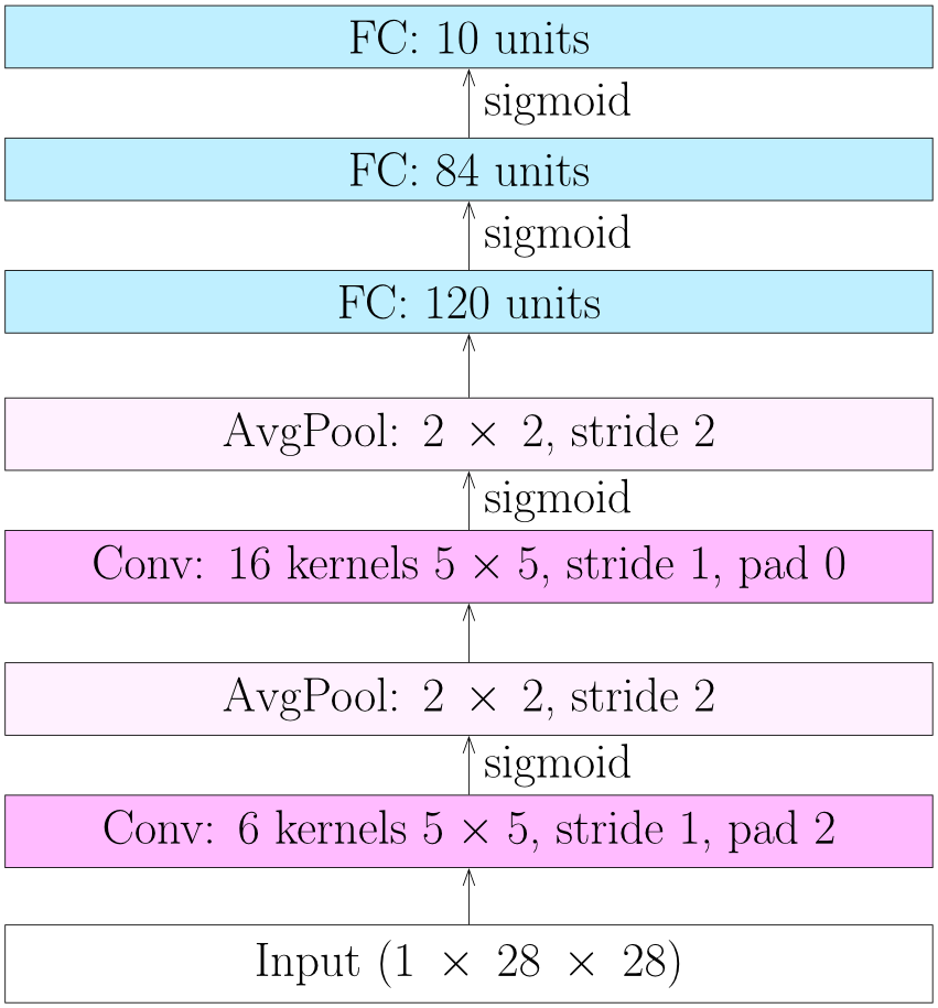
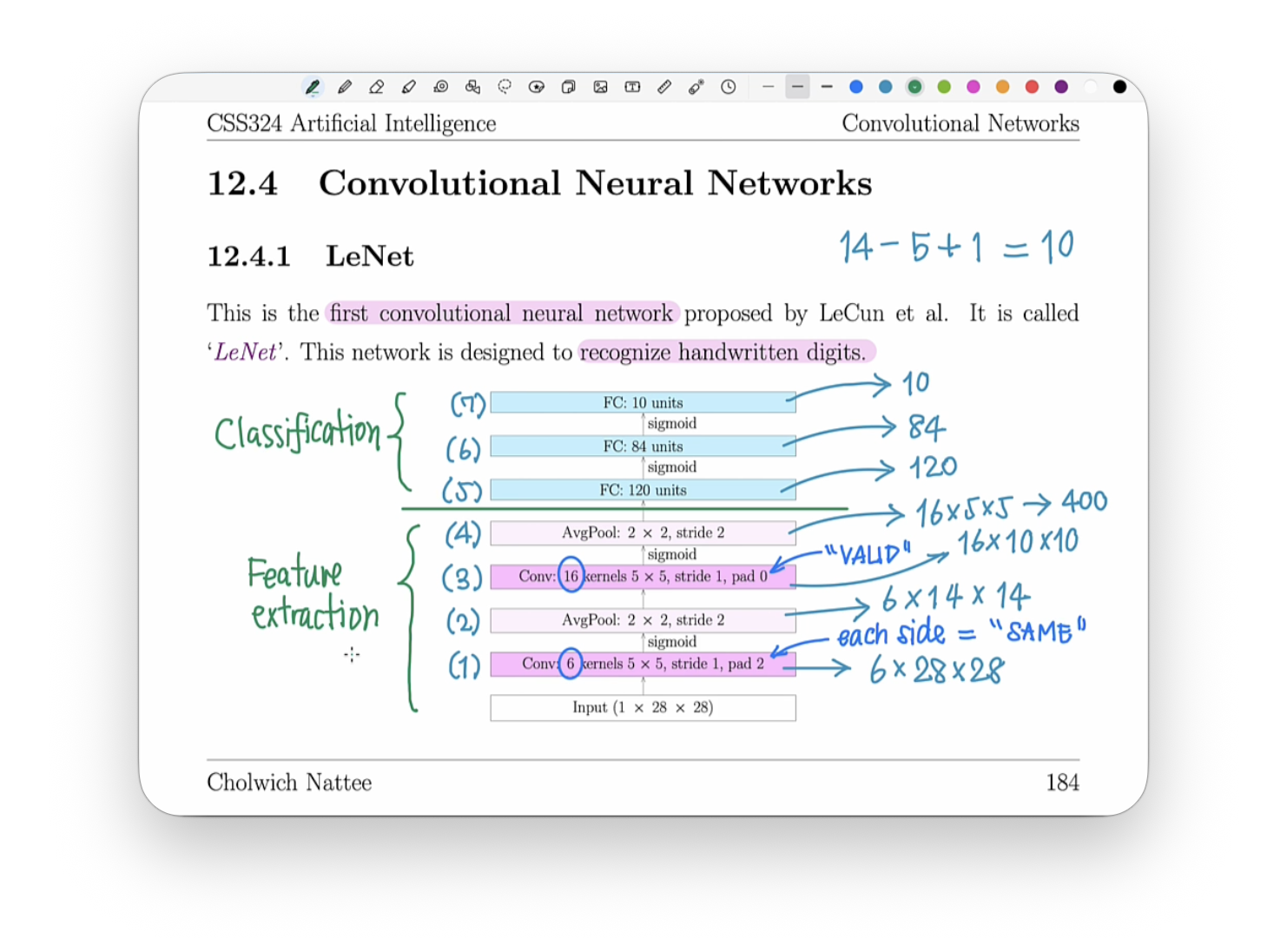
LeNet is the first convolutional neural network proposed by LeCun et al., designed to recognize handwritten digits.

Architecture:

1. Input: $1 \times 28 \times 28$ (grayscale image)
2. Conv Layer 1: 6 kernels $5 \times 5$, stride 1, pad 2, sigmoid
   • pad 2 แปลว่า each side = “SAME convolution”
3. AvgPool Layer 1: $2 \times 2$, stride 2
4. Conv Layer 2: 16 kernels $5 \times 5$, stride 1, pad 0, sigmoid
5. AvgPool Layer 2: $2 \times 2$, stride 2
6. FC Layer 1: 120 units, sigmoid
7. FC Layer 2: 84 units, sigmoid
8. FC Layer 3: 10 units (output), sigmoid

Example 12.11: Parameter Count in LeNet

To calculate the total number of parameters:

• Conv Layer 1: $6\times 5 \times 5 + 6 = 156$ parameters
• Pool = 0
• Conv Layer 2: $16\times5\times5 + 16 = 2,416$ parameters
• Pool = 0
• FC Layer 1: $400\times120+120 = 48,120$ parameters
• FC Layer 2: $120\times 84 + 84$ = 10,164$ parameters
• FC Layer 3: $84 \times 10 +10= 850$ parameters
• Total parameters: ~61,706 parameters

Analogy: LeNet was groundbreaking because it showed that neural networks could learn to recognize patterns in images automatically, much like how you learned to recognize letters without someone explicitly programming rules for each letter shape.

12.4.2 ImageNet Large Scale Visual Recognition Challenge (ILSVRC)

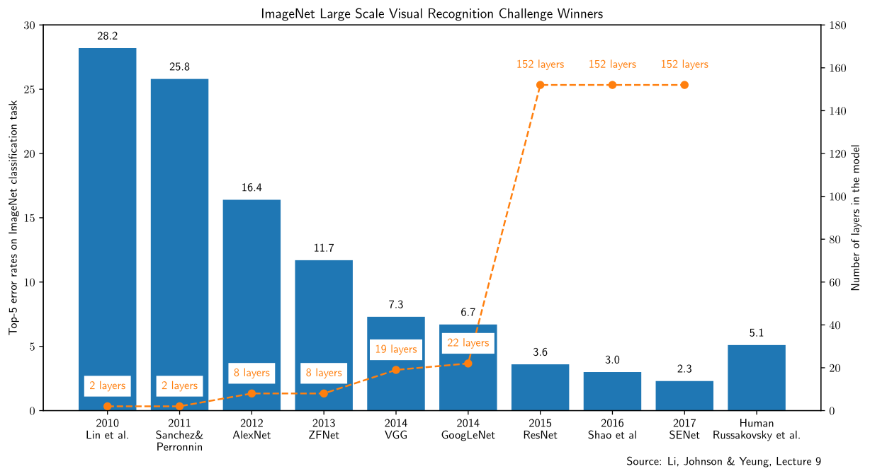
• 2012 คือ ปีที่ Convolutional Neural Network introduced!

ILSVRC is an annual visual recognition competition:

• Goal: Classify objects in images
• Dataset: 1.2 million images with 1,000 classes
• Metric: Top-5 error rate (is correct label in top 5 predictions?)

Progress Over Years:

• 2010: Lin et al. - 28.2% error (2 layers)
• 2011: Sanchez & Perronnin - 25.8% error (2 layers)
• 2012: AlexNet - 16.4% error (8 layers) - Breakthrough with deep learning
• 2013: ZFNet - 11.7% error (8 layers)
• 2014: VGG - 7.3% error (19 layers)
• 2014: GoogLeNet - 6.7% error (22 layers)
• 2015: ResNet - 3.6% error (152 layers)
• 2016: Shao et al. - 3.0% error (152 layers)
• 2017: SENet - 2.3% error (152 layers)
• Human Performance: ~5.1% error

Key Observation: Networks became progressively deeper, with error rates dropping below human performance by 2015.

Analogy: The ILSVRC is like the Olympics of computer vision. Each year, researchers compete to build the best image recognition system, and we've watched as these systems went from mediocre to superhuman in just 7 years.

12.4.3 AlexNet

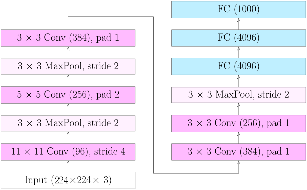
AlexNet (2012) is one of the first deep convolutional neural networks for the ImageNet challenge.

Architecture:

1. Input: $224 \times 224 \times 3$ (RGB image)
2. Conv1: $11 \times 11$ Conv (96 filters), stride 4, ReLU
3. MaxPool1: $3 \times 3$, stride 2
4. Conv2: $5 \times 5$ Conv (256 filters), pad 2, ReLU
5. MaxPool2: $3 \times 3$, stride 2
6. Conv3: $3 \times 3$ Conv (384 filters), pad 1, ReLU
7. Conv4: $3 \times 3$ Conv (384 filters), pad 1, ReLU
8. Conv5: $3 \times 3$ Conv (256 filters), pad 1, ReLU
9. MaxPool3: $3 \times 3$, stride 2
10. FC1: 4096 units, ReLU, Dropout
11. FC2: 4096 units, ReLU, Dropout
12. FC3: 1000 units (output)

Key Innovations:

1. Larger Kernels

• Uses $11 \times 11$ kernel in the first layer
• Necessary to cope with larger images in ImageNet dataset (224×224 vs 28×28 in MNIST)

2. ReLU Activation

• LeNet used sigmoid activation
• AlexNet switched to ReLU (Rectified Linear Unit)
• Benefits: Faster training, helps with vanishing gradient problem

3. Dropout

• Used in fully-connected layers to handle overfitting
• Randomly drops neurons during training

4. Representation Learning

• Lower layers automatically discover features from raw data
• Higher layers represent larger structures
• Network learns hierarchical features

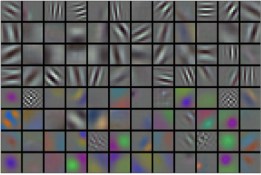
Learned Filters:

• First layer filters learn to detect edges, colors, and simple textures
• Each filter specializes in detecting different low-level features

Analogy: AlexNet is like a hierarchical organization. The first layer employees (filters) handle simple tasks like sorting mail by color. Middle management combines this into "letters vs packages." Top executives make the final decision about what the object is. Each level builds on the work below it.

12.4.4 Visual Geometry Group (VGG) Network

Motivation:

• CNNs are composed of sequences of: convolution layer (with padding + nonlinear activation) → pooling layer (stride 2)
• Each pooling layer reduces resolution by half
• Maximum number of layers is $\log_2 d$ where $d$ is input dimension
• However, deeper networks perform significantly better

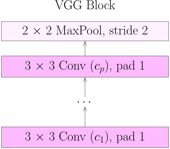
Solution: The VGG Block

VGG Block Structure:

A VGG Block consists of:

1. A sequence of convolution layers with $3 \times 3$ kernels and padding of 1
2. A max pooling layer with $2 \times 2$ window and stride of 2

Notation:

• $c_1, c_2, \ldots, c_p$ = number of channels for each conv layer in the block

VGG Network Structure:

• Sequence of VGG blocks with increasing number of channels
• Followed by 3 fully-connected layers for classification

VGG-16 Example:

• Block 1: 2 conv layers × 64 channels
• Block 2: 2 conv layers × 128 channels
• Block 3: 3 conv layers × 256 channels
• Block 4: 3 conv layers × 512 channels
• Block 5: 3 conv layers × 512 channels
• Total: 16 weight layers (13 conv + 3 FC)

Key Insights:

• Uses only small $3 \times 3$ kernels throughout
• Multiple $3 \times 3$ convolutions have larger receptive field than single large kernel
• More activation functions = more non-linearity = better learning capacity
• Fewer parameters than using large kernels

Analogy: VGG's approach is like reading a book chapter by chapter instead of trying to understand the whole book at once. Small $3 \times 3$ filters are like reading sentences - when you stack them deep enough, you eventually understand complex concepts, just as multiple conv layers build up understanding of complex visual patterns.

12.4.5 Residual Networks (ResNet)

Problem with Very Deep Networks:

• Typically: $\boldsymbol{a}^{[l]} = g^{[l]}(\boldsymbol{W}^{[l]}\boldsymbol{a}^{[l-1]} + \boldsymbol{b}^{[l]})$
• Output at layer $l$ completely replaces output at layer $l-1$
• All layers must learn to keep meaningful information while introducing new information
• This becomes harder as networks get deeper (vanishing/exploding gradients)

ResNet Solution: Skip Connections

Instead of completely replacing representations:

$\boxed{\boldsymbol{a}^{[l]} = g_r^{[l]}(\boldsymbol{a}^{[l-1]} + g^{[l]}(\boldsymbol{W}^{[l]}\boldsymbol{a}^{[l-1]} + \boldsymbol{b}^{[l]}))}$

where $g_r^{[l]}$ is the activation function for the $l$-th residual layer.

Key Idea: A layer should perturb (modify) the representation from the previous layer instead of replacing it completely.

Analogy: Traditional networks are like rewriting an entire essay from scratch each time you want to improve it. ResNet is like editing - you keep what's good and just make small changes (residuals). This makes it much easier to create very deep networks because each layer only needs to learn small adjustments.

Residual Block Types:

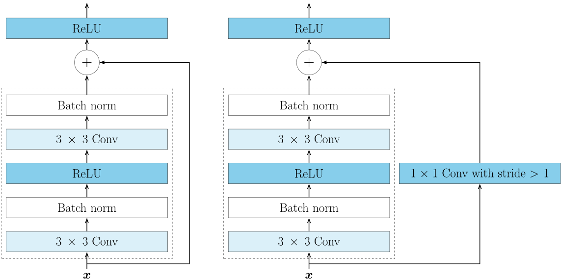
Type 1: Identity Mapping (Same Dimensions)

Input x
   ↓
[3×3 Conv] → [Batch Norm] → [ReLU]
   ↓
[3×3 Conv] → [Batch Norm]
   ↓
   + ← (x added via skip connection)
   ↓
[ReLU]
   ↓
Output

Type 2: With Dimension Adjustment

Input x
   ↓                           ↓
[3×3 Conv] → [Batch Norm] → [ReLU]    [1×1 Conv, stride>1]
   ↓                           ↓
[3×3 Conv] → [Batch Norm] ────+
   ↓
[ReLU]
   ↓
Output

• The $1 \times 1$ convolutional layer with stride > 1 adjusts array dimensions
• Enables residual connections through upsampling/downsampling

ResNet-18 Architecture:

• 18 layers deep
• Multiple residual blocks
• Achieved 3.6% top-5 error on ImageNet (2015)
• Revolutionary because it showed networks can be trained very deep (152 layers in ResNet-152)

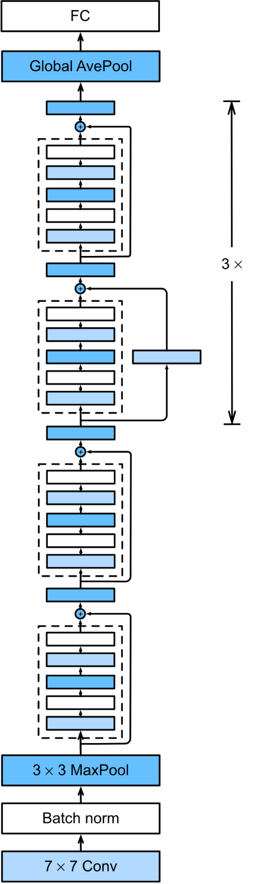
Analogy: Skip connections are like having express lanes on a highway. Information can flow quickly through skip connections (express lane) while also being processed by the layers (regular lanes). This prevents the "traffic jam" of information that happens in very deep traditional networks.

12.3.3 Global Average Pooling

Global Average Pooling averages each feature map (channel) to a single value.

• Input: Array of shape $C \times H \times W$
• Output: Array of shape $C$ (one value per channel)

Process:
For each channel $c$:
$\text{output}_c = \frac{1}{H \times W} \sum_{i=1}^{H} \sum_{j=1}^{W} x_{c,i,j}$

Example 12.12

Input of shape $3 \times 2 \times 2$:

$\left[\begin{bmatrix} 0.1 & 0.1 \\ 0.1 & 0.2 \end{bmatrix}, \begin{bmatrix} 0.2 & 0.8 \\ 0.9 & 0.8 \end{bmatrix}, \begin{bmatrix} 0.7 & 0.9 \\ 0.3 & 0.4 \end{bmatrix}\right]$

Output:

• Channel 1: $(0.1 + 0.1 + 0.1 + 0.2) / 4 = 0.125$
• Channel 2: $(0.2 + 0.8 + 0.9 + 0.8) / 4 = 0.675$
• Channel 3: $(0.7 + 0.9 + 0.3 + 0.4) / 4 = 0.575$

Result: $[0.125, 0.675, 0.575]$

Benefits:

• Reduces overfitting compared to fully connected layers
• No parameters to learn
• Enforces correspondence between feature maps and categories

Analogy: Global Average Pooling is like getting the "general impression" from each feature map. Instead of remembering every detail, you just remember the average level of each feature across the entire image. It's like rating a movie on a scale of 1-10 instead of describing every scene.

12.5 Transfer Learning

Transfer learning reuses a pre-trained model for a new but related task, leveraging learned patterns and features.

Use Case: When labeled data for the new task is limited.

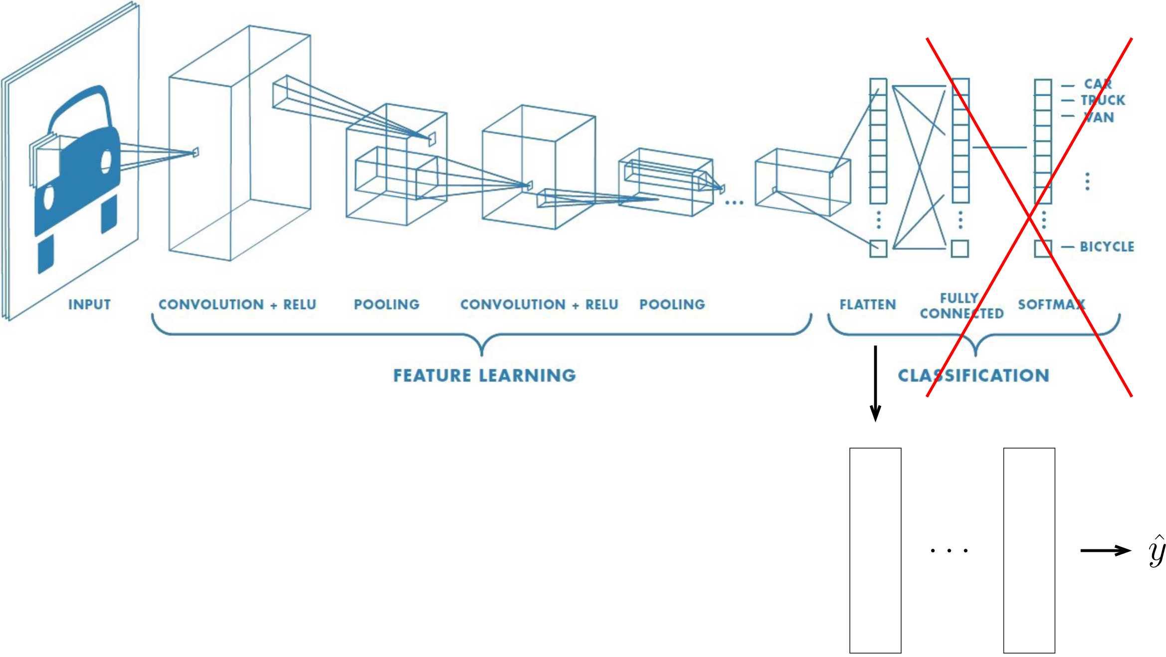
Transfer Learning Process:

1. Pre-trained Model

• A model is first trained on a large, general-purpose dataset
• Learns to extract relevant features (e.g., edges, textures, shapes)

2. Fine-tuning

The pre-trained model is adapted for the new task:

Option A: Replace Classification Layer

• Keep feature extraction layers
• Replace final classification layer with new one for new task
• Train only the new layer

Option B: Freeze Early Layers

• Freeze early layers to retain generic features
• Only retrain later layers on new data

Option C: Fine-tune All Layers

• Retrain entire network on new data
• Use smaller learning rate to preserve learned features

3. Application

• The fine-tuned model is used for the new task

Visual Representation:

[Pre-trained CNN Feature Extraction Layers]
          ↓
    (Frozen or Fine-tuned)
          ↓
[Remove Original Classification Layer]
          ↓
[Add New Classification Layer for New Task]
          ↓
     [Train on New Dataset]

Advantages:

• Requires less training data for new task
• Faster training (leveraging pre-learned features)
• Often achieves better performance than training from scratch
• Especially useful when new dataset is small

Common Pre-trained Models:

• ResNet (trained on ImageNet)
• VGG (trained on ImageNet)
• Inception (trained on ImageNet)

Analogy: Transfer learning is like hiring an experienced photographer to shoot weddings instead of teaching someone photography from scratch. The photographer already knows about lighting, composition, and camera settings (general features). They just need to learn the specific requirements for weddings (task-specific features). This is much faster than teaching someone everything from zero.

Practical Example:

• Pre-trained model: ResNet trained on ImageNet (1000 object categories)
• New task: Classify 10 types of medical images
• Process: Keep ResNet feature extraction, replace final layer with 10-class classifier, train on medical images
• Result: Good performance even with limited medical image data

Summary of Key Concepts

Why CNNs?

• Preserve spatial relationships in images
• Share weights across locations (translation invariance)
• Reduce parameters compared to fully connected networks

Core Operations:

• Convolution/Cross-correlation: Extract local features
• Pooling: Downsample and extend receptive field
• Activation: Introduce non-linearity (ReLU most common)

Architecture Evolution:

1. LeNet (1998): First CNN, 7 layers, handwritten digits
2. AlexNet (2012): 8 layers, ImageNet breakthrough, introduced ReLU and dropout
3. VGG (2014): 16-19 layers, uniform 3×3 kernels, deeper is better
4. ResNet (2015): 152 layers, skip connections, superhuman performance

Modern Techniques:

• Transfer Learning: Reuse pre-trained models for new tasks
• Batch Normalization: Stabilize training
• Data Augmentation: Improve generalization
• Global Average Pooling: Reduce overfitting

Practice Problems

Problem 1: Output Shape Calculation

Given an input of shape $32 \times 32 \times 3$, calculate the output shape after:

• Conv layer: 64 kernels of size $5 \times 5$, stride 1, padding 2
• MaxPool: $2 \times 2$, stride 2

Problem 2: Parameter Counting

Calculate the number of parameters in a conv layer with:

• Input channels: 3
• Output channels: 64
• Kernel size: $7 \times 7$
• Include bias

Problem 3: Receptive Field

What is the receptive field size at the 3rd convolutional layer if:

• All kernels are $3 \times 3$
• All strides are 1
• No pooling layers

Problem 4: Design Decision

You're building a CNN for a new image classification task with limited data. Should you:

• Train from scratch?
• Use transfer learning?
• Explain your reasoning.

Additional Notes

Important Formulas Summary:

Cross-correlation output size (valid):
$\boxed{(n_h - k_h + 1) \times (n_w - k_w + 1)}$

Padding for same convolution:
$\boxed{p = l - 1}$

Output size with stride:
$\boxed{\left\lfloor \frac{n_h - k_h + p_h + s_h}{s_h} \right\rfloor \times \left\lfloor \frac{n_w - k_w + p_w + s_w}{s_w} \right\rfloor}$

Receptive field (stride 1):
$\boxed{(l - 1)m + 1}$

Parameters in conv layer:
$\boxed{(k_h \times k_w \times c_{in} + 1) \times c_{out}}$

Tips for Success

When Designing CNNs:

1. Start with proven architectures (ResNet, VGG)
2. Use $3 \times 3$ kernels (most efficient)
3. Add batch normalization
4. Use dropout in FC layers
5. Try transfer learning first

Common Mistakes to Avoid:

• Forgetting to add padding (output shrinks)
• Using too large kernels (too many parameters)
• Not using batch normalization
• Training from scratch with small datasets
• Ignoring data augmentation

Debugging Checklist:

• Check input/output dimensions match
• Verify learning rate isn't too high
• Ensure data is normalized
• Check for data leakage
• Monitor both training and validation loss