Overview
Spark Streaming is a framework for large-scale stream processing that enables processing of live data streams with near-real-time latency.
Key Capabilities
- Scalability: Scales to hundreds of nodes
- Low Latency: Can achieve second-scale latencies
- Integration: Integrates with Spark's batch and interactive processing
- Simple API: Provides a batch-like API for implementing complex algorithms
- Data Sources: Can absorb live data streams from Kafka, Flume, ZeroMQ, TCP sockets, etc.
Real-world Analogy: Think of Spark Streaming like a conveyor belt in a factory that processes items in small batches rather than one at a time. Instead of stopping the belt to process each item individually, you group items into small batches and process them together - this is faster and more efficient.
Motivation
Why Stream Processing?
Many important applications must process large streams of live data and provide results in near-real-time:
- Social network trends (e.g., Twitter trending topics)
- Website statistics (real-time analytics)
- Intrusion detection systems (security monitoring)
- Real-time recommendations
Requirements
- Large clusters to handle workloads
- Latencies of few seconds (not milliseconds, but not minutes either)
Production Example: Netflix uses stream processing to:
- Track which shows users are watching in real-time
- Generate personalized recommendations instantly
- Monitor video quality issues across millions of streams
- Detect anomalies in user behavior for fraud prevention
Case Study: Conviva, Inc.
Problem Statement
Real-time monitoring of online video metadata for major networks (HBO, ESPN, ABC, SyFy, etc.)
The Two-Stack Problem
Before Spark Streaming, companies like Conviva needed two separate processing stacks:
-
Custom-built distributed stream processing system
- Processes 1000s of complex metrics on millions of video sessions
- Requires many dozens of nodes for processing
- Provides real-time monitoring
-
Hadoop backend for offline analysis
- Generates daily and monthly reports
- Similar computation as the streaming system (duplicate code!)
The Headache 😫
- 2× the effort to implement any new function
- 2× the bugs to solve
- 2× the headache maintaining two codebases
- 2× the infrastructure costs
Real-world Impact: Imagine having to write every feature twice - once for real-time processing and once for batch reports. This is what companies faced before unified frameworks like Spark Streaming.
Requirements for a Streaming Framework
Core Requirements
- ✅ Scalable to large clusters
- ✅ Second-scale latencies
- ✅ Simple programming model (Spark programming with Scala and RDDs)
- ✅ Integrated with batch & interactive processing
- ✅ Efficient fault-tolerance in stateful computations
Scalability Factors
What determines scalability?
- ⏱️ Minimized Latency Rate
- 💻 Computation cost
- 💾 Storage cost
- 🌐 Communication cost
- 📊 Throughput
- 🛡️ Fault tolerance
The Challenge: Stateful Stream Processing
Traditional Streaming Systems
Traditional streaming systems use an event-driven record-at-a-time processing model:
[Input Records] → [Node 1 with Mutable State] → [Node 2 with Mutable State] → [Node 3]
How it works:
- Each node has mutable state
- For each record, the node:
- Updates its state
- Sends new records downstream
The Problem ❌
- State is lost if node dies!
- Making stateful stream processing fault-tolerant is challenging
Existing Solutions and Their Issues
Storm
- ✅ Replays records if not processed by a node
- ⚠️ Processes each record at least once
- ❌ May update mutable state twice (double counting!)
- ❌ Mutable state can be lost due to failure
Trident
- ✅ Uses transactions to update state
- ✅ Processes each record exactly once
- ❌ Per-state transaction updates are slow
Real-world Problem: Imagine counting website visitors in real-time. If Storm crashes and replays some records, you might count the same visitor twice. For a bank processing transactions, double-counting would be catastrophic!
Spark Streaming Solution
Core Concept: Discretized Stream Processing
Key Idea: Run a streaming computation as a series of very small, deterministic batch jobs
[Live Data Stream] → [Batch X seconds] → [Spark Streaming]
                                               ↓
                                          [RDD Processing]
                                               ↓
                                        [Processed Results]
                                               ↓
                                            [Spark]
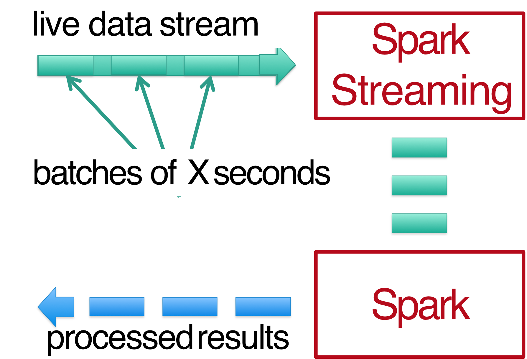
How It Works
- Chop up the live stream into batches of X seconds
- Spark treats each batch of data as RDDs
- Process using RDD operations
- Return processed results in batches
Performance Characteristics
- Batch sizes: As low as ½ second
- Latency: ~1 second
- Benefit: Potential for combining batch and streaming processing in the same system
Real-world Analogy: Instead of processing each email as it arrives (which is inefficient), Spark Streaming is like processing emails in small batches every second. You still get near-instant results, but with much better efficiency.
Key Concepts
1. DStream (Discretized Stream)
DStream = A sequence of RDDs representing a stream of data
val tweets = ssc.twitterStream(<username>, <password>)Time: t t+1 t+2
DStream: [RDD] → [RDD] → [RDD] → ...
||| ||| |||
Nodes Nodes Nodes
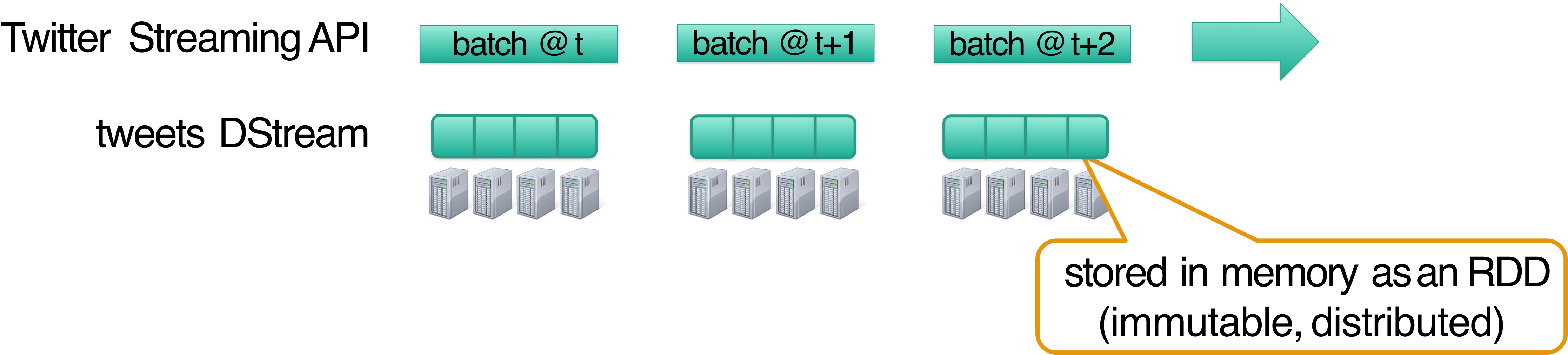
Each batch is stored in memory as an RDD (immutable, distributed)
Data Sources:
- Twitter Streaming API
- HDFS
- Kafka
- Flume
- ZeroMQ
- Akka Actor
- TCP sockets
2. Transformations
Transformations modify data from one DStream to create another DStream
val hashTags = tweets.flatMap (status => getTags(status))Standard RDD Operations
map()- Transform each elementflatMap()- Transform each element to multiple elementsfilter()- Keep elements matching conditioncountByValue()- Count occurrences of each valuereduce()- Aggregate elementsjoin()- Combine two streamscogroup()- Group data from multiple streams
Stateful Operations
window()- Sliding window over timecountByValueAndWindow()- Count over windowreduceByKeyAndWindow()- Reduce over windowupdateStateByKey()- Maintain arbitrary state
3. Output Operations
Output Operations send data to external storage
saveAsHadoopFiles()- Save to HDFSforeachRDD()- Apply arbitrary operations to each batch
Map vs FlatMap
Understanding the Difference
- Map: Applied to each element in the RDD → one new value per input element
- FlatMap: Applied to each element in the RDD → zero, one, or more values per input element (then flattened)
Example: Splitting Sentences into Words
# Input RDD
lines = sc.parallelize([
    "Apache Spark is fast",
    "Spark is powerful"
])
Using map()
lines.map(lambda x: x.split(" ")).collect()

# Output: [
#   ['Apache', 'Spark', 'is', 'fast'],
#   ['Spark', 'is', 'powerful']
# ]
# Result is RDD of lists
Using flatMap()
lines.flatMap(lambda x: x.split(" ")).collect()

# Output: ['Apache', 'Spark', 'is', 'fast', 'Spark', 'is', 'powerful']
# Result is RDD of individual elements (flattened)
Why FlatMap?
Each input line produces multiple output elements (words), and flatMap flattens them into a single list.
Practice Exercise
nums = sc.parallelize([1, 2, 3])

# Map
nums.map(lambda x: (x, x*x)).collect()
# Output: [(1, 1), (2, 4), (3, 9)]

# FlatMap
nums.flatMap(lambda x: (x, x*x)).collect()
# Output: [1, 1, 2, 4, 3, 9]
Key Insight:
mappreserves structure (one-to-one), whileflatMapallows one-to-many transformations and flattens the result.
Example 1: Get Hashtags from Twitter
Scala Code
val tweets = ssc.twitterStream(<username>, <password>)
val hashTags = tweets.flatMap(status => getTags(status))
hashTags.saveAsHadoopFiles("hdfs://...")
Visual Flow
Time:           t           t+1          t+2

tweets      [RDD]  →    [RDD]   →    [RDD]   →  ...
              ↓           ↓            ↓
           flatMap     flatMap      flatMap
              ↓           ↓            ↓
hashTags    [RDD]  →    [RDD]   →    [RDD]   →  ...
              ↓           ↓            ↓
            save        save         save
              ↓           ↓            ↓
            [HDFS]      [HDFS]       [HDFS]
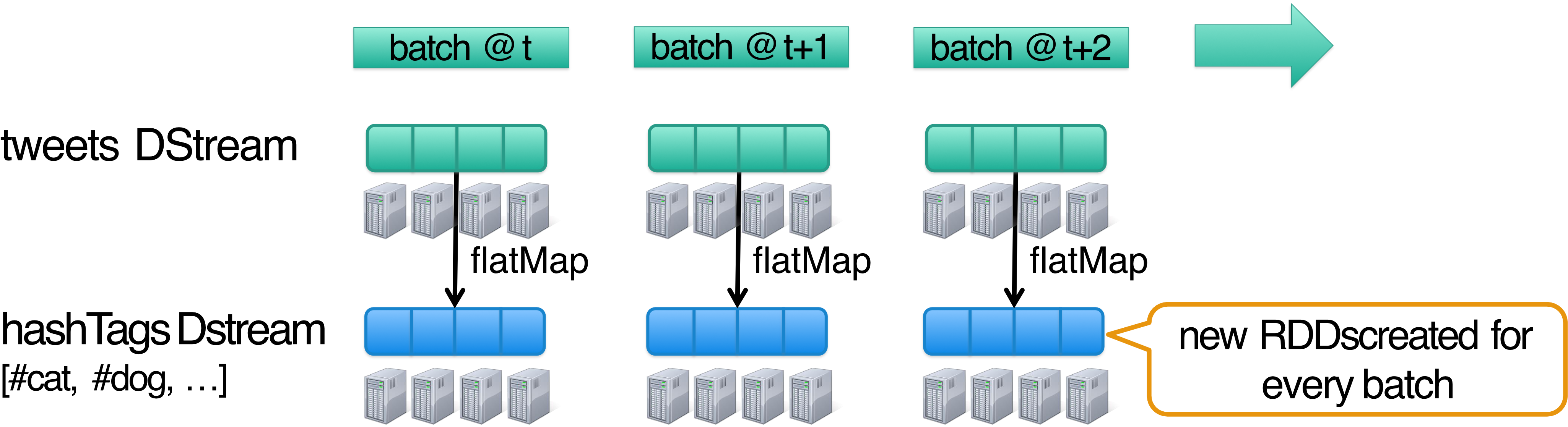
What happens:
- New RDDs created for every batch
- Each batch is stored in memory as an immutable, distributed RDD
- Output operation (
save) pushes data to external storage (HDFS)
Java Example
// Scala
val tweets = ssc.twitterStream(<username>, <password>)
val hashTags = tweets.flatMap(status => getTags(status))
hashTags.saveAsHadoopFiles("hdfs://...")

// Java
JavaDStream<Status> tweets = ssc.twitterStream(<username>, <password>)
JavaDStream<String> hashTags = tweets.flatMap(new Function<...> { })
hashTags.saveAsHadoopFiles("hdfs://...")
Java requires a Function object to define the transformation (more verbose than Scala).
Production Example: Twitter uses similar stream processing to:
- Track trending hashtags in real-time
- Detect breaking news as it happens
- Monitor platform health and user engagement
- Filter spam and inappropriate content
Example 2: Count the Hashtags
Code
val tweets = ssc.twitterStream(<username>, <password>)
val hashTags = tweets.flatMap(status => getTags(status))
val tagCounts = hashTags.countByValue()
Visual Flow
Time:        t            t+1           t+2

tweets     [RDD]   →    [RDD]    →    [RDD]   →  ...
             ↓            ↓             ↓
          flatMap      flatMap       flatMap
             ↓            ↓             ↓
hashTags   [RDD]   →    [RDD]    →    [RDD]   →  ...
             ↓            ↓             ↓
           map          map           map
             ↓            ↓             ↓
        reduceByKey  reduceByKey   reduceByKey
             ↓            ↓             ↓
tagCounts  [RDD]   →    [RDD]    →    [RDD]   →  ...
        [(#cat,10),  [(#dog,25),   [(#ai,50),
         (#dog,25)]   (#cat,15)]    (#ml,30)]
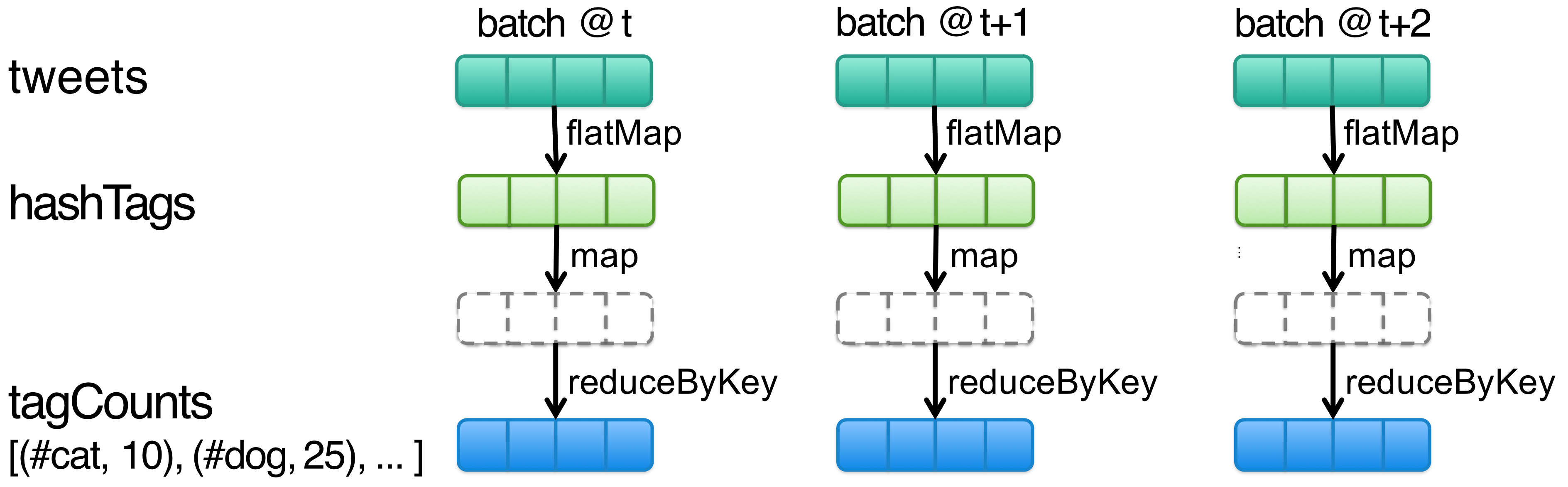
What countByValue() does internally:
- Map each element to (element, 1)
- ReduceByKey to sum up counts
Real-world Usage: This is exactly how social media platforms show you trending topics with their popularity counts in real-time!
Example 3: Count Hashtags Over Last 10 Minutes (Sliding Window)
Code
val tweets = ssc.twitterStream(<username>, <password>)
val hashTags = tweets.flatMap(status => getTags(status))
val tagCounts = hashTags.window(Minutes(10), Seconds(1))
                        .countByValue()
Components
- Window Length:
Minutes(10)- Look at last 10 minutes of data - Sliding Interval:
Seconds(1)- Compute new results every 1 second
Visual Flow
Time:       t-1     t      t+1     t+2     t+3

hashTags    [●]    [●]    [●]     [●]     [●]   →  ...
              └──────┴──────┴──────┘
                 Sliding Window
                       ↓
                  countByValue
                       ↓
                   [Result]
                  (count over all
                   data in window)
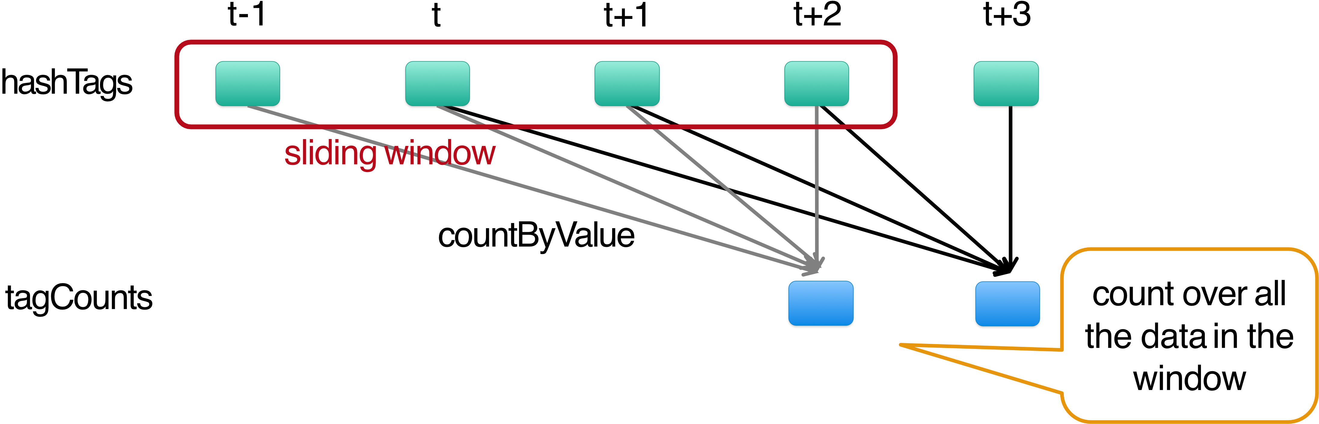
The window slides forward every second, always looking at the last 10 minutes of data.
Real-world Example: This is how YouTube's "Trending Now" section works - it shows videos that are popular in a recent time window, updated continuously.
Smart Window-Based CountByValue
The Problem with Naive Window Operations
Naive approach: Recompute counts for all data in the window every time
- ❌ Inefficient: Re-processing all data every second
- ❌ Expensive: Lots of redundant computation
The Smart Solution: Incremental Computation
val tagCounts = hashTags.countByValueAndWindow(Minutes(10), Seconds(1))How It Works
Time:       t-1     t      t+1     t+2     t+3

hashTags    [●]    [●]    [●]     [●]     [●]   →  ...
             ↓      ↓      ↓       ↓
        countByValue|      |       |
             ↓      |      |       |
tagCounts   [5]    [7]    [9]    [10]    [12]  →  ...
             │       └──────┴───────┴──────┘
             │              │       │       │
             │              ↓       ↓       ↓
             └─────────→  [OLD] → [+NEW] → [RESULT]
                          Subtract  Add
                          (batch    (batch
                          before    in
                          window)   window)
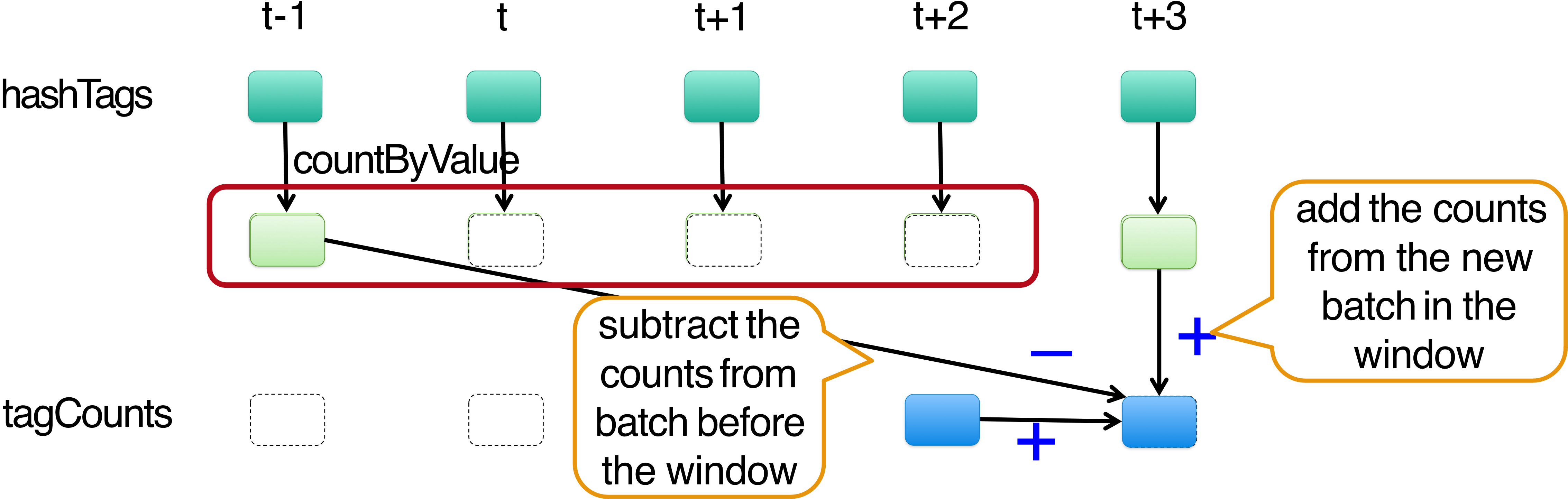
The Incremental Algorithm
Steps:
- Start with previous window's count
- Subtract counts from batch leaving the window
- Add counts from new batch entering the window
- Result: Updated count with minimal computation!
Smart Window-Based Reduce
This technique generalizes to many reduce operations:
hashTags.reduceByKeyAndWindow(
    _ + _,  // Function to add new data
    _ - _,  // Function to remove old data (inverse reduce)
    Minutes(10),
    Seconds(1)
)
Need a function to "inverse reduce" (e.g., subtraction for addition, division for multiplication)
Performance Benefit: Instead of processing 600 batches (10 minutes of data at 1-second intervals) every second, you only process 2 batches (one leaving, one entering). This is a 300× efficiency improvement!
Example 4:
- มาเขียนด้วยเด้ออ
- สำคัญนะะ ทำความเข้าใจด้วยนะ Sliding Window
Spark Join Operation
What is Join?
Join in Spark SQL is the functionality to join two or more datasets similar to table joins in SQL-based databases.
Syntax
def join[W](other: RDD[(K, W)]): RDD[(K, (V, W))]Example
val rdd1 = sc.makeRDD(Array(("A","1"), ("B","2"), ("C","3")), 2)
val rdd2 = sc.makeRDD(Array(("A","a"), ("C","c"), ("D","d")), 2)

rdd1.join(rdd2).collect()

// Result: Array[(String, (String, String))]
//       = Array((A,(1,a)), (C,(3,c)))
Explanation:
- Only keys present in both RDDs appear in result
- Values from both RDDs are combined into tuples
- This is an inner join by default
Production Usage:
- Netflix: Join user viewing data with content metadata
- Uber: Join rider requests with driver locations
- E-commerce: Join order data with inventory data
Cogroup Operation
- Last #MidtermExam นะ ออก Cogroup, แต่บอกว่าเทอมนี้ไม่แน่ใจว่าจะออกอะไร
What is Cogroup?
cogroup() is a transformation function on PairRDD that groups data from multiple RDDs by key.
For each key k: Return a tuple with lists of all values for that key from each RDD.
Example
Input PairRDDs:
[(A,1), (B,1), (C,1), (D,1)]
[(B,2), (D,2)]

Result of cogroup:
[(A,{1}), (B,{1,2}), (C,1), (D,{1,2})]
Key Points:
- Returns key + iterable lists of values from each RDD
- Includes keys even if they only appear in one RDD
- Like a full outer join but with grouped values
Use Case: Cogroup is perfect when you want to process all related data together, like combining user profile data from multiple sources.
Fault Tolerance
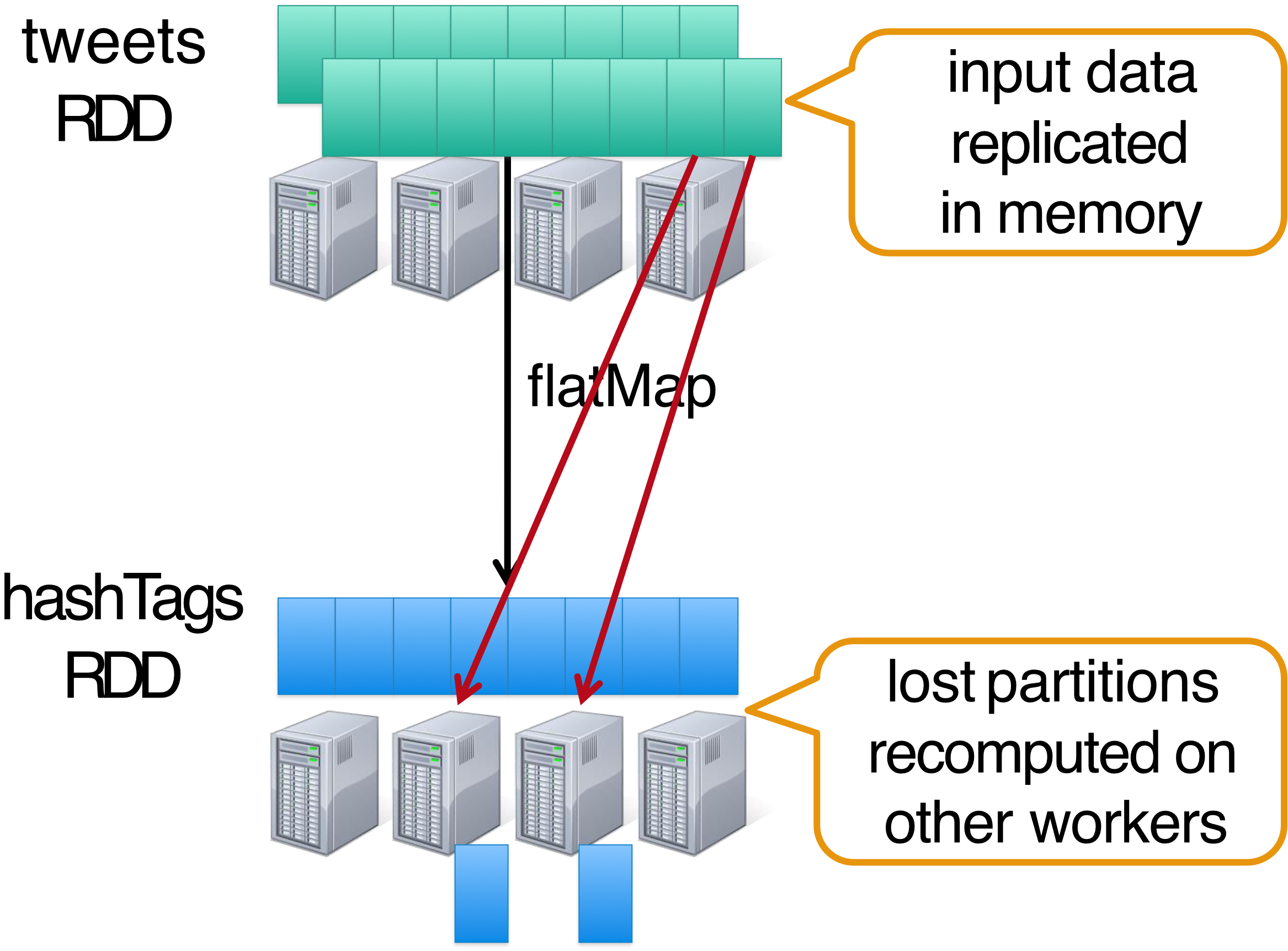
How Spark Streaming Achieves Fault Tolerance
1. RDD Lineage
RDDs remember the sequence of operations that created them from the original fault-tolerant input data.
Input Data (replicated) → flatMap → map → reduce → Output
     ↑
  Stored in
  memory on
multiple nodes
They remember it as lineage metadata (DAG) stored in the Spark Driver’s memory (DAG) + Worker nodes.
2. Input Data Replication
Batches of input data are replicated in memory of multiple worker nodes → fault-tolerant
3. Lost Data Recovery
If a worker fails:
- Input data is still available (replicated)
- Lost RDD partitions can be recomputed from input data using lineage
- Computation is deterministic → same input → same output
Visual Example
tweets RDD    [Node1] [Node2] [Node3] [Node4]
                 ↓       ↓       ↓       ✗ (failed)
              flatMap  flatMap flatMap
                 ↓       ↓       ↓
hashTags RDD  [Node1] [Node2] [Node3] [Node4]
                 ↓       ↓       ↓       ↑
                 └───────────────────────┘
                   Recompute on other nodes
                   using replicated input
Exactly-Once Semantics
- State data not lost even if a worker node dies
- Immutable RDDs: Does not change the value of your result
- Exactly once semantics to all transformations
- ✅ No double counting!
Why This Matters: In financial applications, you can't afford to count a transaction twice or lose a transaction. Spark Streaming's fault tolerance guarantees correct results even with failures.
Performance Benchmarks
Scalability
Can process 6 GB/sec (60M records/sec) on 100 nodes at sub-second latency
Test Setup:
- 100 streams of data
- 100 EC2 instances with 4 cores each
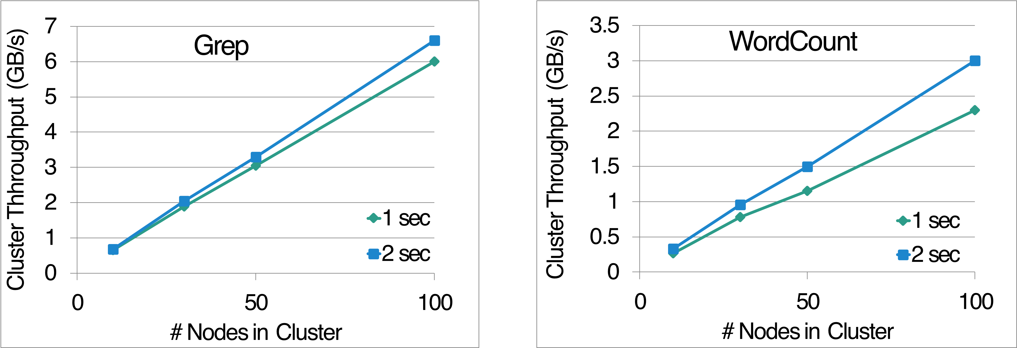
Grep Performance
Nodes:        20    50    100
Throughput:
  1 sec:     2     3.5    6.5   GB/s
  2 sec:     2     3.2    6     GB/s
WordCount Performance
Nodes:        20    50    100
Throughput:
  1 sec:     0.5   1.5    3     GB/s
  2 sec:     0.4   1.2    2.4   GB/s
Key Insight: Near-linear scalability with number of nodes!
Comparison with Storm and S4
Throughput per Node:
Grep (100-byte records)
- Spark Streaming: ~65 MB/s per node
- Storm: ~12 MB/s per node
- Ratio: Spark is 5-6× faster
WordCount (100-byte records)
- Spark Streaming: ~27 MB/s per node
- Storm: ~6 MB/s per node
- Ratio: Spark is 4-5× faster
Overall Performance
- Spark Streaming: 670k records/second/node
- Storm: 115k records/second/node
- Apache S4: 7.5k records/second/node
Fast Fault Recovery
Recovers from faults/stragglers within 1 second
Processing Time Graph:
│
2.0 │          Failure Happens
│              ↓
1.5 │  ████████████████████████████████
│  ████████████████████████████████
1.0 │  ████████████████████████████████
│  ████████████████████████████████
0.5 │  ████████████████████████████████
│
0.0 └─────────────────────────────────→ Time
    0   15   30   45   60   75   90

Sliding WordCount on 10 nodes with 30s checkpoint interval
Red bars show recovery period - barely noticeable impact!
Production Impact: For a system processing millions of events per second, 1-second recovery means you lose at most a few million events, which can be replayed from the source. Traditional systems might take minutes to recover, losing hundreds of millions of events.
Vision: One Stack to Rule Them All
The Unified Processing Stack
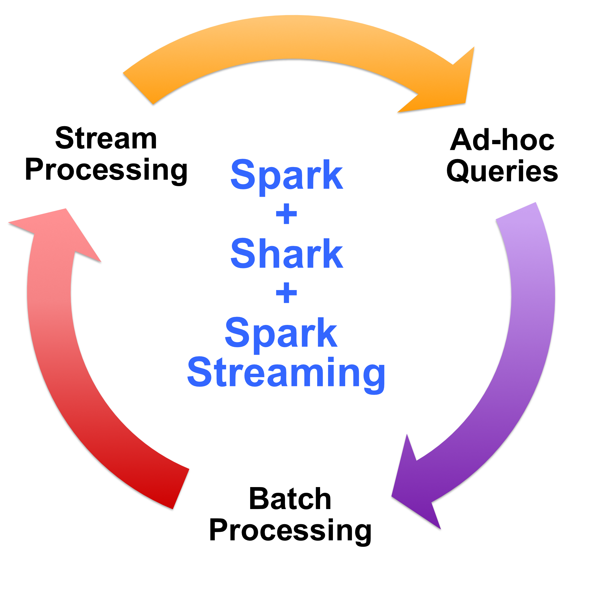
Benefits of Unified Stack
1. Code Reuse Across Modes (SKIPPED)
Interactive Exploration (Spark Shell):
$ ./spark-shell
scala> val file = sc.hadoopFile("smallLogs")
scala> val filtered = file.filter(_.contains("ERROR"))
scala> val mapped = file.map(...)
Batch Processing (Production):
object ProcessProductionData {
  def main(args: Array[String]) {
    val sc = new SparkContext(...)
    val file = sc.hadoopFile("productionLogs")
    val filtered = file.filter(_.contains("ERROR"))
    val mapped = file.map(...)
  }
}
Stream Processing (Real-time):
object ProcessLiveStream {
  def main(args: Array[String]) {
    val sc = new StreamingContext(...)
    val stream = sc.kafkaStream(...)
    val filtered = stream.filter(_.contains("ERROR"))
    val mapped = stream.map(...)
  }
}
2. Workflow Integration
Typical Data Pipeline:
- Explore data interactively using Spark Shell/PySpark to identify problems
- Test with same code in Spark standalone programs on production logs
- Deploy similar code in Spark Streaming to identify problems in live streams
Spark Program vs Spark Streaming Program
Batch (Spark):
val tweets = sc.hadoopFile("hdfs://...")
val hashTags = tweets.flatMap(status => getTags(status))
hashTags.saveAsHadoopFile("hdfs://...")
Streaming (Spark Streaming):
val tweets = ssc.twitterStream(<username>, <password>)
val hashTags = tweets.flatMap(status => getTags(status))
hashTags.saveAsHadoopFiles("hdfs://...")Difference: Only the data source changes! The transformation logic is identical.
Real-world Example: At Uber, engineers use:
- Spark Shell to explore historical ride data and test new features
- Spark Batch Jobs to generate daily/weekly reports
- Spark Streaming to track real-time ride requests and match drivers
Same codebase, same team, same cluster - three different use cases!
Getting Started
Alpha Release
Spark Streaming is available with Spark 3.2.1 and later versions.
Download: https://spark.apache.org/downloads.html
Documentation: PySpark Streaming API
Summary
Spark Streaming is a stream processing framework that is...
✅ Scalable to large clusters
- Horizontal scaling: Add more nodes → process more data
- Tested up to 100+ nodes
✅ Fast
- Achieves second-scale latencies (0.5-2 seconds)
- Throughput: 6 GB/sec on 100 nodes
✅ Simple
- Batch-like programming model
- Familiar RDD operations
- Less code than traditional streaming systems
✅ Integrated
- Works with Spark batch processing
- Works with Spark SQL for ad-hoc queries
- Same codebase for multiple use cases
✅ Fault-tolerant
- Efficient fault-tolerance in stateful computations
- Exactly-once semantics
- Fast recovery (< 1 second)
Resources
📄 Research Paper: http://tinyurl.com/dstreams
Key Takeaways
When to Use Spark Streaming
✅ Use Spark Streaming when:
- You need near-real-time processing (seconds)
- You want to reuse code between batch and streaming
- You need strong fault-tolerance guarantees
- You're already using Spark ecosystem
- You need stateful processing (windows, aggregations)
❌ Don't use Spark Streaming when:
- You need sub-second latency (use Flink or custom solutions)
- Your data rate is very low (simple cron jobs might suffice)
- You only do simple filtering/routing (use Kafka Streams)
Production Best Practices
-
Batch Interval Selection
- Start with 5-10 seconds
- Decrease only if processing can keep up
- Monitor processing time vs batch interval
-
Memory Management
- Enable memory-only storage for frequently accessed data
- Use checkpointing for long windows
- Monitor GC pressure
-
Fault Tolerance
- Enable checkpointing for stateful operations
- Use reliable receivers for data sources
- Test failure scenarios
-
Performance Tuning
- Tune number of partitions
- Enable data locality
- Use serialization (Kryo)
- Optimize window operations (use incremental operations)
Cloud Services Using Spark Streaming
AWS
- Amazon EMR: Managed Spark Streaming clusters
- Amazon Kinesis + Spark: Real-time analytics
- AWS Glue: ETL with Spark Streaming
Google Cloud
- Dataproc: Managed Spark clusters
- Pub/Sub + Dataproc: Event streaming
Azure
- Azure Databricks: Collaborative Spark environment
- Azure HDInsight: Managed Spark Streaming
- Azure Event Hubs + Spark: Real-time ingestion
Databricks
- Delta Live Tables: Production-grade streaming pipelines
- Structured Streaming: Modern streaming API
- Auto Scaling: Dynamic resource allocation
Enterprise Example:
- Netflix processes 500+ billion events/day with Spark Streaming on AWS
- Uber uses Spark Streaming for real-time pricing and fraud detection
- Pinterest processes user engagement data in real-time for recommendations
- Alibaba handles millions of transactions per second during shopping festivals
Glossary
DStream: Discretized Stream - sequence of RDDs representing a stream
RDD: Resilient Distributed Dataset - Spark's core immutable data structure
Batch Interval: Time duration for each micro-batch (e.g., 1 second)
Window Length: How far back to look in time for windowed operations
Sliding Interval: How frequently to compute windowed operations
Checkpointing: Saving state to reliable storage for fault recovery
Exactly-once: Guarantee that each record affects state exactly one time
At-least-once: Record may be processed multiple times (less strict)
Lineage: The sequence of transformations that created an RDD
Fault Tolerance: Ability to recover from failures without data loss