Introduction
- Recurrent Neural Networks (RNNs) are a class of artificial neural networks designed for processing sequential data
- Unlike traditional feed-forward neural networks, RNNs have connections that form directed cycles
- This allows them to maintain a memory of previous inputs in their internal state
- Particularly well-suited for tasks where the order of input data is important:
- Time series analysis
- e.g. Stock prices = sequence of real values
- Natural language processing
- e.g. a sentence = sequence of words (vector นั่นแหละ)
- Speech recognition
- Time series analysis
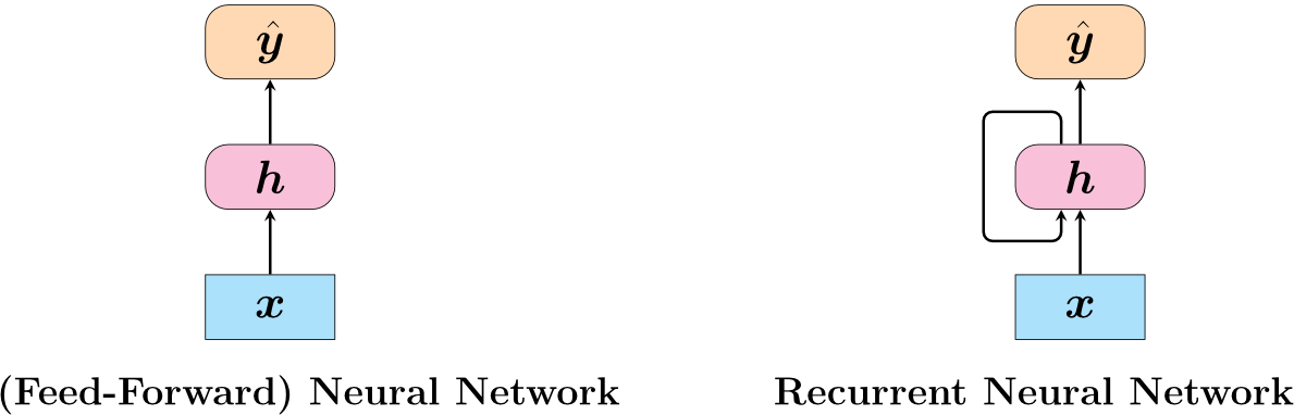
Think of RNNs like reading a book: you remember what happened in previous chapters to understand the current page, unlike feed-forward networks that only look at one page at a time without context.
13.1 Architecture
Basic RNN Structure
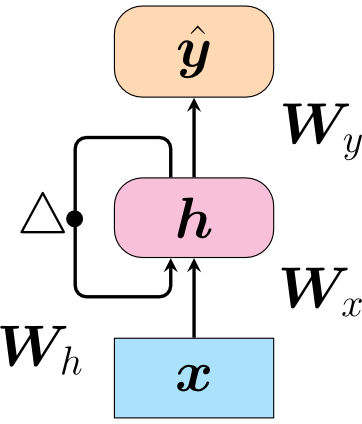
Components:
- Input:
- Hidden State:
- Output:
- Delay operator: (indicates feedback from previous time step)
Key Equations
Hidden state update equation at step :
Output at step :
Where:
- = weight of the input
- = weight of the hidden (feedback) layer
- = weight of the output
- = biases of the hidden layer and output layer, respectively
- = input at step (time)
- = activation function
- = delay operator
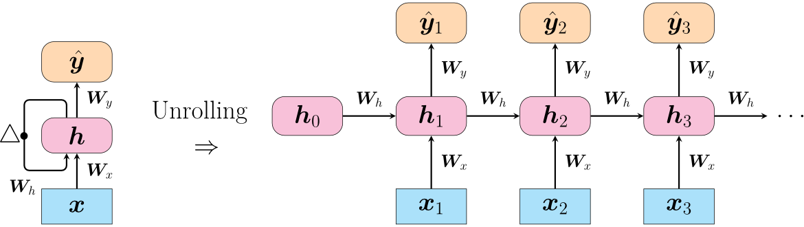
Unrolling RNNs
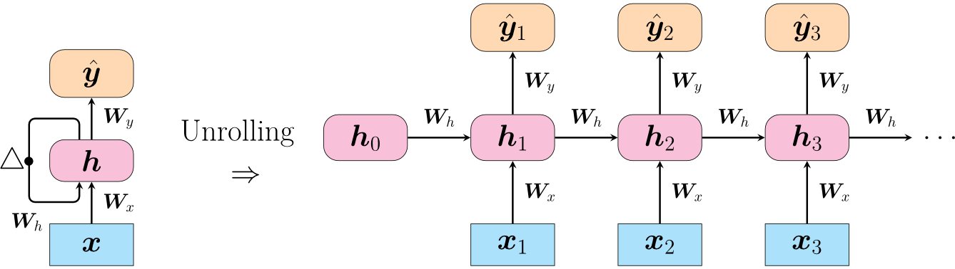
- RNNs can be "unrolled" through time to visualize how they process sequences
- The network is replicated for each time step, with shared weights across all time steps
Unrolled structure:
Key assumptions:
- The hidden state at time () is computed from the current input and the previous hidden state
- The output at time () is computed from the current hidden state
- RNNs make a Markov assumption: the current state depends on a finite fixed number of previous states
Think of unrolling like laying out a film strip: each frame (time step) shows the same camera (network) capturing different moments, but using the same lens settings (shared weights).
Multiple Recurrent Layers
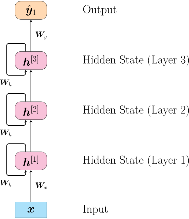
- RNNs can be stacked into multiple layers for deeper representations
- Each layer processes the output of the previous layer
- Notation: represents hidden state at layer and time
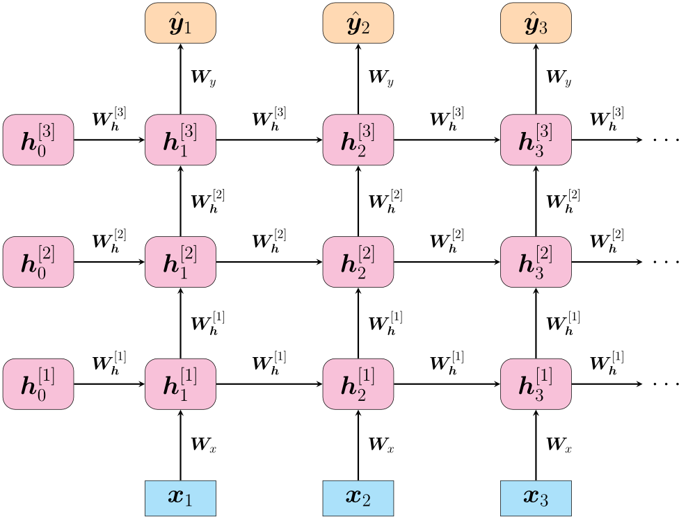
Example structure:
- Input → Hidden Layer 1 → Hidden Layer 2 → Hidden Layer 3 → Output
- Each layer has its own recurrent connections:
13.1.1 Weights and Biases Sharing
Concept
- RNNs share weights and biases across different time steps to maintain consistency
- Regardless of how many times the RNN is unfolded, the number of parameters remains constant
Benefits of Weight and Bias Sharing
- Parameter Efficiency
- Reduces the number of parameters
- Makes the model more efficient and easier to train
- Generalization
- Ensures the model can generalize patterns across different time steps in the sequence
- Temporal Consistency
- Maintains consistency in how inputs and hidden states are processed over time
- Crucial for learning temporal dependencies
Imagine a translator who uses the same grammar rules (shared weights) for every sentence they translate, rather than learning new rules for each sentence. This makes them consistent and efficient.
Example 13.1: Stock Market Price Prediction
Given:
- Stock market prices of Company A over 5 days
- RNN with 1 hidden layer
- Parameters:
- (initial hidden state)
- Identity activation function
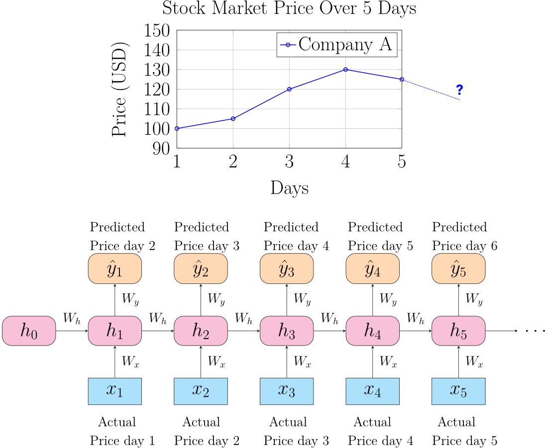
Task: Predict the price of Day 6
Calculation steps:
Day 1:
-
-
- (Not necessary)
- เพราะว่าเราอยากได้ , we need just that! ไม่ต้องเสียเวลาคำนวณ
Day 2:
Day 3:
Day 4:
Day 5:
Day 6:
Day 6 เอามาหลอกเลยเด้อ5555
Thus the predicted price for Day 6 is 117.21
13.1.2 How to Train RNN
Backpropagation Through Time (BPTT)
- To train an RNN, unroll it through time and use regular backpropagation
- This method is called Backpropagation Through Time (BPTT)
Training Steps
- Forward Pass
- Perform the forward pass through the unrolled network
- For each time step, compute the hidden states and outputs using shared weights and biases
- Loss Function
- Use a loss (error) function to evaluate the output against the target values
- Backward Pass (Gradient Calculation)
- The gradients are propagated backwards through the unrolled network:
- a) Output Weight ():
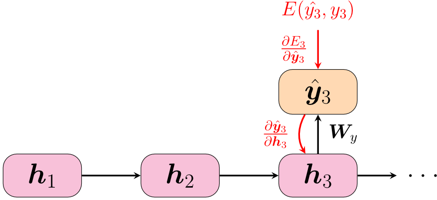
- a) Output Weight ():
- The gradients are propagated backwards through the unrolled network:
where is the time step of the interested output
- b) Input Weight ():
Important note:
- Since , we cannot treat as a constant
- The gradient from time step is calculated using the gradient from time step
- Requires recursive calculation
c) Hidden (Recurrent) Weight ():
Important note:
- Similar to , we cannot treat as a constant
- The gradient calculation requires recursive computation through all previous time steps
Think of BPTT like tracing back your steps: if you made a wrong turn (error) at the end of a journey, you need to walk back through all your previous steps to figure out where you first went wrong.
- Parameter Update
- Update the model parameters using the gradients computed during BPTT
- Repeat
- Continue the process until convergence
13.1.3 Vanishing and Exploding Gradients Problem in RNNs
อาจจะมีปัญหาเกิดขึ้นได้ 2 อย่าง
The Problem
- RNNs maintain a hidden state that gets updated at each time step
- Update rule:
Gradient Flow Analysis
During BPTT, we compute gradients of the loss function with respect to network parameters:
Key term to understand:
Let . The gradient with respect to the hidden state at time step is:
This recursive multiplication can cause two major problems:
1. Vanishing Gradients
Condition: If the eigenvalues of are less than 1 in magnitude
Mathematical expression:
- For small eigenvalues of , approaches zero as increases
- Gradients shrink exponentially as they propagate backward through time
Consequence:
- The model is unable to learn long-term dependencies
- Gradients are too small to make significant updates to the weights for earlier time steps
Like a whisper being passed through a long line of people: by the time it reaches the last person, the message has faded to almost nothing.
2. Exploding Gradients
Condition: If the eigenvalues of are greater than 1 in magnitude
Mathematical expression:
- For large eigenvalues of , increases exponentially as increases
- Gradients grow exponentially as they propagate backward through time
Consequence:
- The model's training becomes unstable
- Parameters update too drastically
- Leads to divergence or oscillations in the loss function
Like a snowball rolling down a mountain: it starts small but grows uncontrollably large, eventually causing an avalanche.
13.2 Long Short-Term Memory (LSTM)
Overview
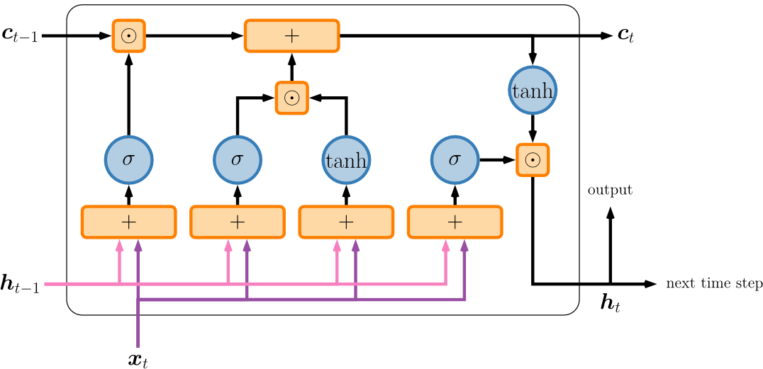
- LSTM is a type of RNN architecture designed to address the vanishing gradient problem
- Introduced to enable learning of long-term dependencies in sequential data
- Uses a sophisticated gating mechanism to control information flow
13.2.1 LSTM Cell Structure
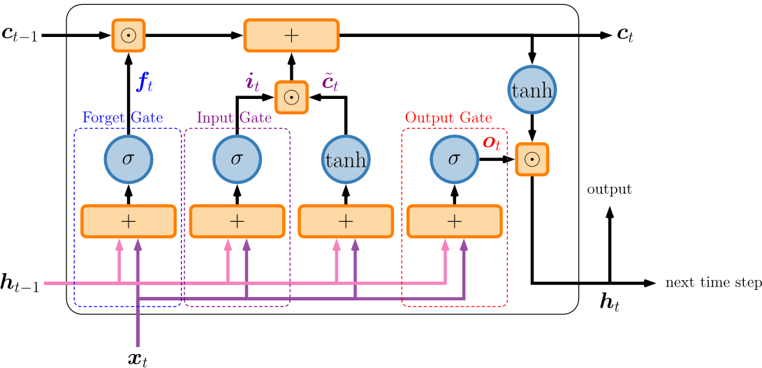
An LSTM cell consists of three main components:
1. Gates
Gates control the flow of information in the LSTM cell.
a) Forget Gate ()
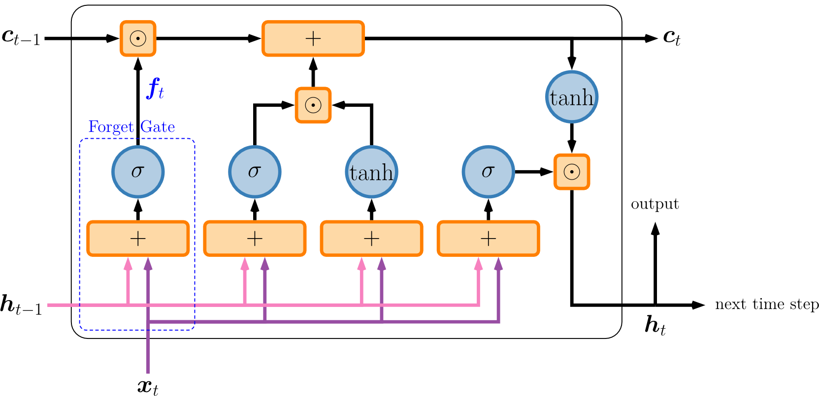
- Purpose: Decides what information to discard from the cell state
- Formula:
Think of the forget gate as a filter that decides which old memories to throw away, like forgetting what you had for breakfast last week.
- ถ้า Close to 0, discard, แต่ถ้า close to 1, it will change to 1
- = element-wise multiplication
b) Input Gate ()
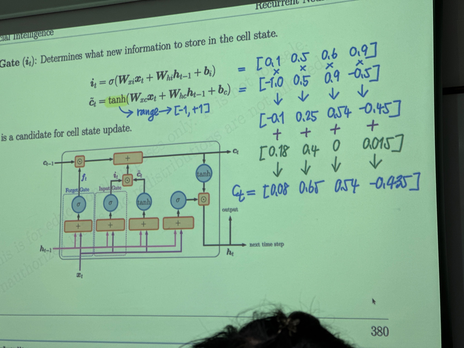
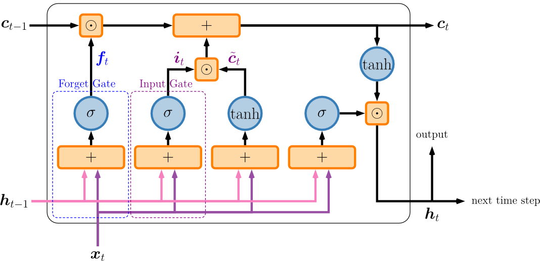
- Purpose: Determines what new information to store in the cell state
- Formulas:
Note: is a candidate for cell state update
The input gate acts like a security checkpoint, deciding which new information is important enough to remember.
c) Output Gate ()
- Purpose: Controls the output and the contribution of the cell state to the hidden state
- Formula:
The output gate decides what information from your memory to actually use right now, like choosing which facts to recall for an exam.
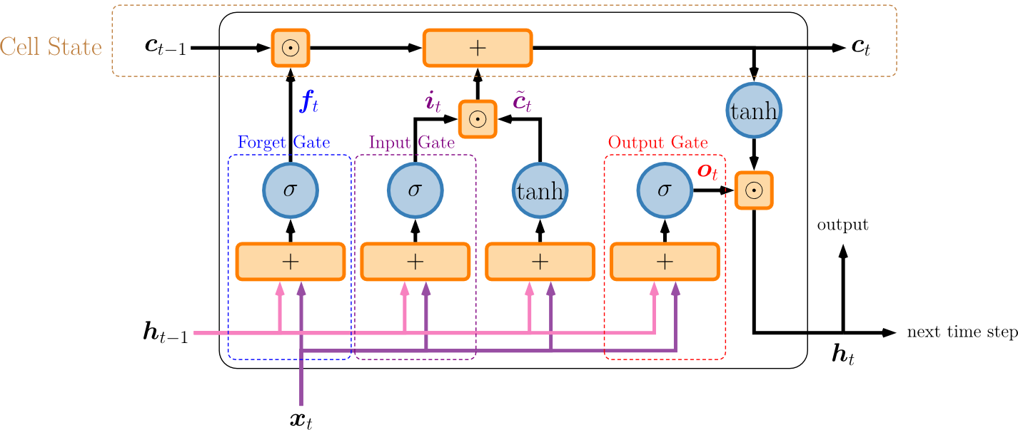
2. Cell State ()
- The cell state is the memory of the LSTM cell
- Carries information across different time steps
- Modified by the gates
- Update formula (where is element-wise multiplication):
Interpretation:
- : Keep parts of old memory based on forget gate
- : Add new information based on input gate
The cell state is like a conveyor belt running through the entire chain, with gates adding or removing information along the way.
3. Hidden State ()
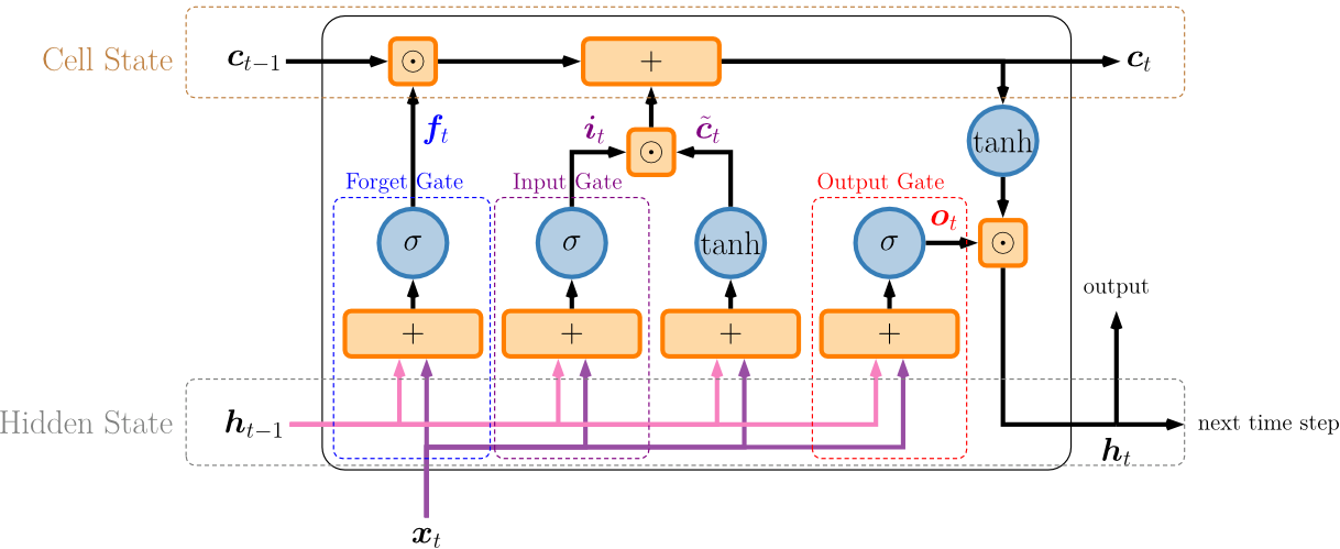
- The hidden state is the output of the LSTM cell at each time step
- Used for predicting the next output
- Serves as input to the LSTM cell in the next time step
- Update formula:
The hidden state is your short-term working memory, focusing on what's immediately relevant from your long-term memory (cell state).
Key Distinction
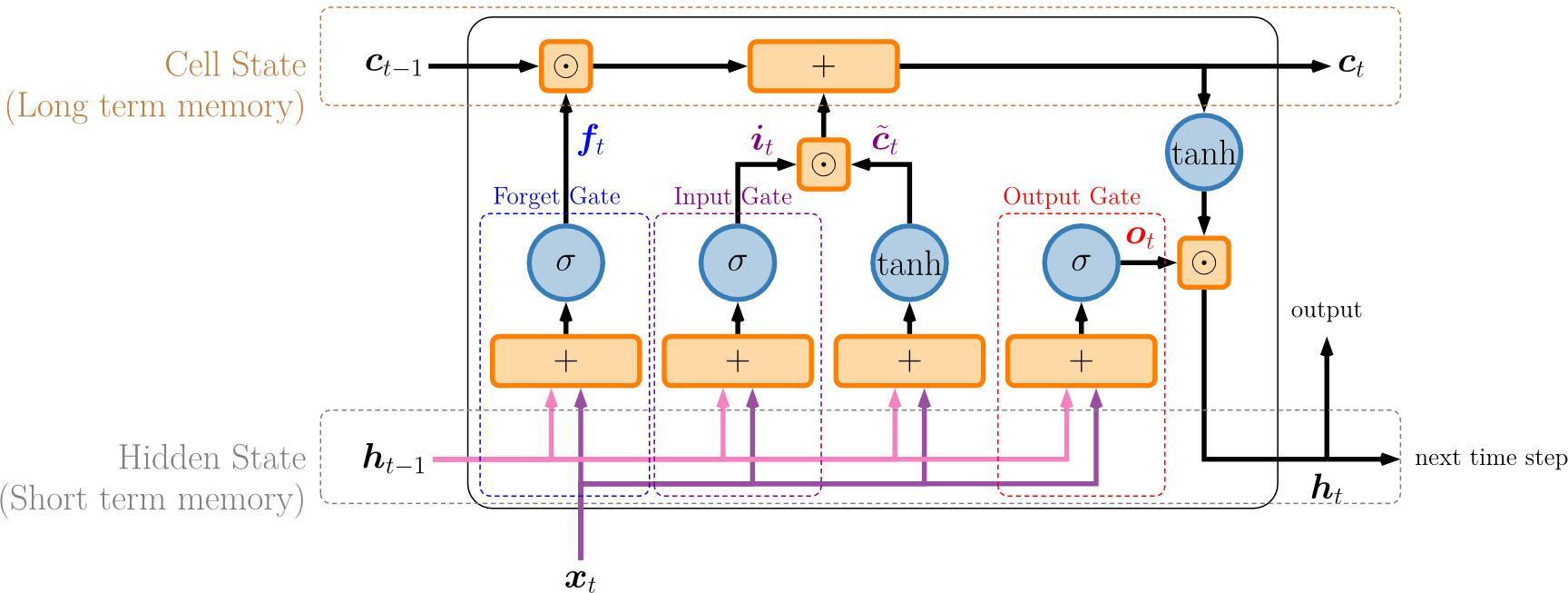
- Cell State (): Long-term memory
- Hidden State (): Short-term memory
13.2.2 LSTM Workflow
Step-by-Step Process
- Input
- At each time step , the LSTM cell receives:
- Current input:
- Previous hidden state:
- At each time step , the LSTM cell receives:
- Gates Computation
- The forget, input, and output gates are computed to control information flow
- Cell State Update
- Cell state is updated based on:
- Forget gate
- Input gate
- Candidate cell state
- Cell state is updated based on:
- Hidden State Update
- Hidden state is updated based on:
- Cell state
- Output gate
- Hidden state is updated based on:
- Output
- The hidden state serves as:
- Output of the LSTM cell
- Input for the next time step
- The hidden state serves as:
Visual Summary
13.2.3 Example 13.2: LSTM Calculation
Given
Input:
Parameters:
- Weights:
- Weights:
- Biases:
- Initial hidden state:
- Initial cell state:
Task: Calculate
Time Step t = 1
Forget Gate:
Input Gate:
Candidate Cell State:
Cell State Update:
Output Gate:
Hidden State:
Time Step
Forget Gate:
Input Gate:
Candidate Cell State:
Cell State Update:
Output Gate:
Hidden State:
From the given sequence
[1,0.5], the calculated LSTM states are
- At ,
- At ,
The final output is
13.2.3 How LSTM Solves the Vanishing Gradient Problem
Constant Error Carousel (CEC)
- The cell state enables the constant flow of error through the network during backpropagation
- Gradients can pass through many time steps without diminishing significantly
- This is the primary mechanism that addresses vanishing gradients
Why it works:
- The cell state update uses additive operations rather than multiplicative:
- The gradient can flow through the addition operation without being repeatedly multiplied by weight matrices
- This preserves gradient magnitude over long sequences
Imagine a highway (cell state) where information can travel quickly without traffic lights (no repeated multiplications). This prevents the signal from getting weaker over long distances.
Gate Mechanism
- The gates (forget, input, output) control the amount of information flowing in and out of the cell state
- Ensures that important information is retained over long sequences
- Protects against both vanishing and exploding gradients by regulating information flow
Key advantages:
- Selective memory: Forget gate discards irrelevant information
- Selective updates: Input gate chooses what new information to add
- Selective output: Output gate controls what to use from memory
13.2.4 How LSTM Solves the Exploding Gradient Problem
While vanishing gradients are more common, LSTMs also help with exploding gradients:
1. Gradient Clipping
- Although not specific to LSTMs, gradient clipping is often used alongside LSTMs
- Technique that prevents gradients from becoming excessively large
- Sets a threshold: if gradient exceeds it, scale it down
2. Regulated Flow of Information
- The gates in LSTMs regulate the flow of information
- Prevents uncontrolled growth of gradients
- Controls input and output at each time step through sigmoid activations (bounded between 0 and 1)
Why it works:
- Gate values are bounded:
- Prevents explosive growth through multiplication
- Provides stable training dynamics
Summary
LSTMs effectively address both gradient problems through:
- Architecture design: Cell state with additive updates
- Gating mechanism: Controlled information flow
- Combined techniques: Gradient clipping when needed
This makes LSTMs well-suited for various sequence modeling tasks requiring long-term dependencies.
Think of LSTM gates as a smart thermostat: they keep the temperature (gradient) in a comfortable range, preventing it from getting too cold (vanishing) or too hot (exploding).
13.3 Transformer Model
- seq2seq model e.g. machine translation
Overview
- Transformer model introduced by Vaswani et al. in "Attention is All You Need" (2017)
- Revolutionary architecture that changed NLP and sequence modeling
- Key innovation: Relies entirely on self-attention mechanism
- Does not use recurrence like RNNs and LSTMs
- Draws global dependencies between input and output
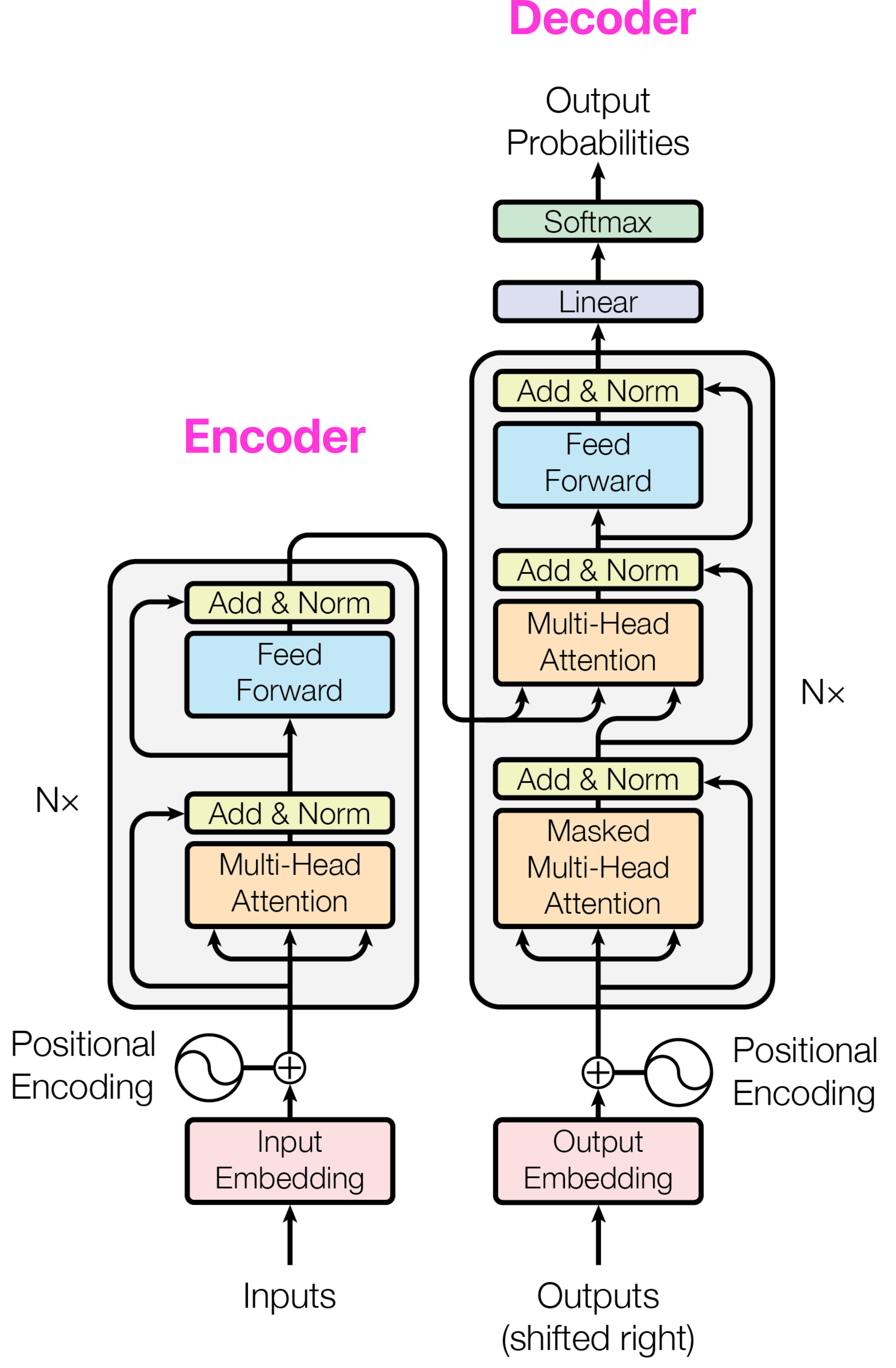
13.3.1 Self-Attention Mechanism
Overview
- Self-attention is the key innovation of the Transformer model
- Allows each position in the input sequence to attend to all other positions
- Enables parallel processing (unlike sequential RNNs)
How Self-Attention Works
Step 1: Linear Projections
Input embeddings are linearly transformed into three vectors:
- Queries (Q): What am I looking for?
- Keys (K): What do I contain?
- Values (V): What information do I carry?
Formulas:
where is the input matrix and are learned weight matrices.
ก็เอาไปผ่าน Layer Neural Network เหมือนคำนวณออกมาชั้นนึง
Step 2: Scaled Dot-Product Attention
Formula:
- บางครั้ง () เรียกว่า Contextualized representation
where:
- = dimension of the key vectors
- = scaled dot product (attention scores)
- = attention weights
- Final output = weighted sum of values
Why scaling by ?
- Prevents dot products from getting too large
- Keeps gradients stable during training
- Helps softmax function work in optimal range
Think of attention like a search engine: Queries are your search terms, Keys are webpage titles, and Values are the actual content. The mechanism finds which pages (Keys) match your search (Query) and returns relevant content (Values).
Step 3: Multi-Head Attention
- Uses multiple self-attention heads simultaneously
- Each head learns to focus on different aspects of the input
- Outputs are concatenated and linearly transformed
Formula:
where:
Benefits:
- Model can jointly attend to information from different representation subspaces
- Different heads can focus on different types of relationships (e.g., syntactic, semantic)
- Increases model's expressive power
Multi-head attention is like having multiple expert readers analyze a text simultaneously: one focuses on grammar, another on meaning, another on context, and their insights are combined.
Self-Attention for Long-Range Dependencies
- Self-attention allows the model to capture long-range dependencies
- Each word can directly attend to every other word in the sequence
- No need to pass information through many intermediate steps (unlike RNNs)
Example visualization:
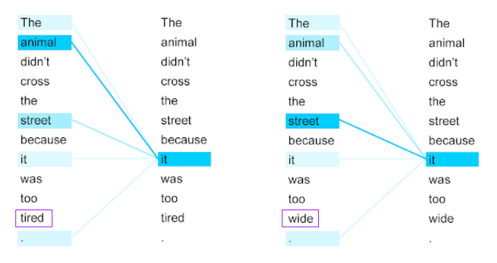
-
When processing the word "it" in "The animal didn't cross the street because it was too tired"
-
Self-attention can directly connect "it" to "animal" regardless of distance
-
Different attention heads might connect different word pairs
-
แต่ละ Words ฝั่งซ้าย represented by
- งั้นถ้าความหมายเหมือนกัน 100% คำว่า it ทั้งสองฝั่งก็ต้องเหมือนกัน เท่ากัน 100% สิ
- เรา Calculate
attentionจาก it ฝั่งขวา เพื่อหา Stronger attention- แต่ละ Attention notation คือ
- สุดท้ายคำนวณ ซึ่งค่าของ ทั้งสองฝั่งก็จะไม่เท่ากันละ!
Scaled Dot-Product Attention Process (Detailed)
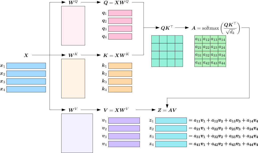
Given: Input sequence
Step 1: Create Q, K, V matrices
Step 2: Compute attention scores
Step 3: Apply scaling and softmax
- ดังนั้น Each row รวมกันจะได้ 1 ไง
Step 4: Compute weighted sum of values
where:
13.3.2 Key Components of the Transformer
The Transformer consists of two main components:
High-Level Architecture
┌─────────────┐  Z    ┌─────────────┐
│   Encoder   │  -->  │   Decoder   │
└─────────────┘       └─────────────┘
      ↑                      ↓
 x = "How are you?"   Y = "お元気ですか。"
   (Input)               (Output)
Encoder:
- Processes the input sequence
- Produces a matrix representation ( or ) of the input
- Example: English sentence "How are you?" → encoded representation
Decoder:
- Takes the encoded representation
- Generates output step by step (autoregressively)
- Example: Translates to Japanese "お元気ですか。"
Both encoder and decoder consist of a stack of identical layers.
Encoder Architecture
The encoder converts input tokens into contextualized representations.
Components
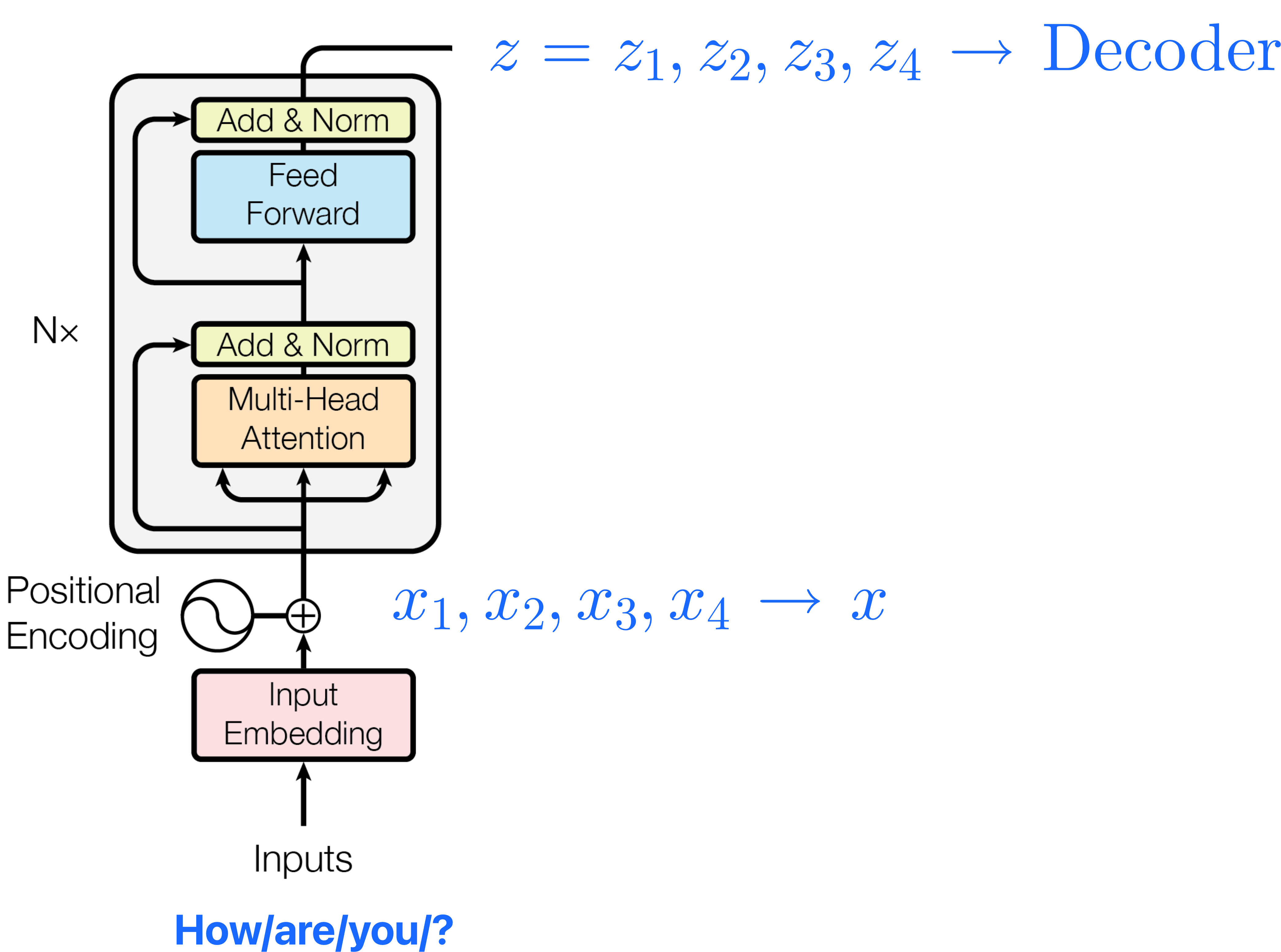
1. Input Embedding
- Converts input tokens into semantic vectors using embedding layers
- Each token becomes a dense vector representation
2. Positional Encoding
- Adds positional information to embeddings using sine and cosine functions
- Enables the model to track token order (since attention has no inherent notion of position)
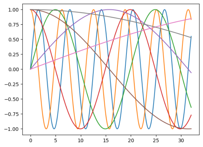
Formula:
where:
- = position in sequence
- = dimension index
- = model dimension
Positional encoding is like adding timestamps to messages so the model knows which came first, even when processing them all at once.
3. Stack of Encoder Layers
The original Transformer uses N = 6 identical encoder layers. Each layer contains:
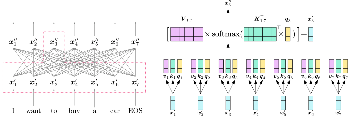
3.1 Multi-Head Self-Attention Mechanism
Purpose: Allows the model to focus on different parts of the input
Process:
- Matrix multiplication of queries and keys to create score matrix
- Scaling down scores for stable gradients: divide by
- Apply softmax function to obtain attention weights
- Multiply softmax weights by value vectors to produce output
- Pass through linear layer
Multi-head aspect:
- Splits Q, K, V into multiple heads
- Each head processes independently
- Outputs are combined and fine-tuned
- Enriches model with diverse understanding
3.2 Normalization and Residual Connections
- Each sub-layer is followed by:
- Layer normalization: Stabilizes training
- Residual connection: Adds input directly to output
Formula:
Benefits:
- Helps build deeper models
- Reduces vanishing gradient problem
- Enables better gradient flow
3.3 Feed-Forward Neural Network
- Point-wise feed-forward network applied to each position
- Two linear layers with ReLU activation in between
Formula:
- Applied identically to each position separately
- Followed by residual connection and normalization
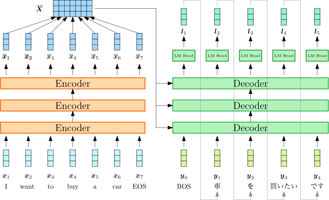
4. Output of Encoder
-
BOS = Beginning of sentence
-
Final encoder layer outputs context-rich vectors representing the input
-
These vectors serve as input to the decoder
-
Guide decoder to focus on relevant words during generation
-
By stacking N layers, model gains:
- Deeper understanding
- Different aspects of attention
- Stronger predictive power
Decoder Architecture
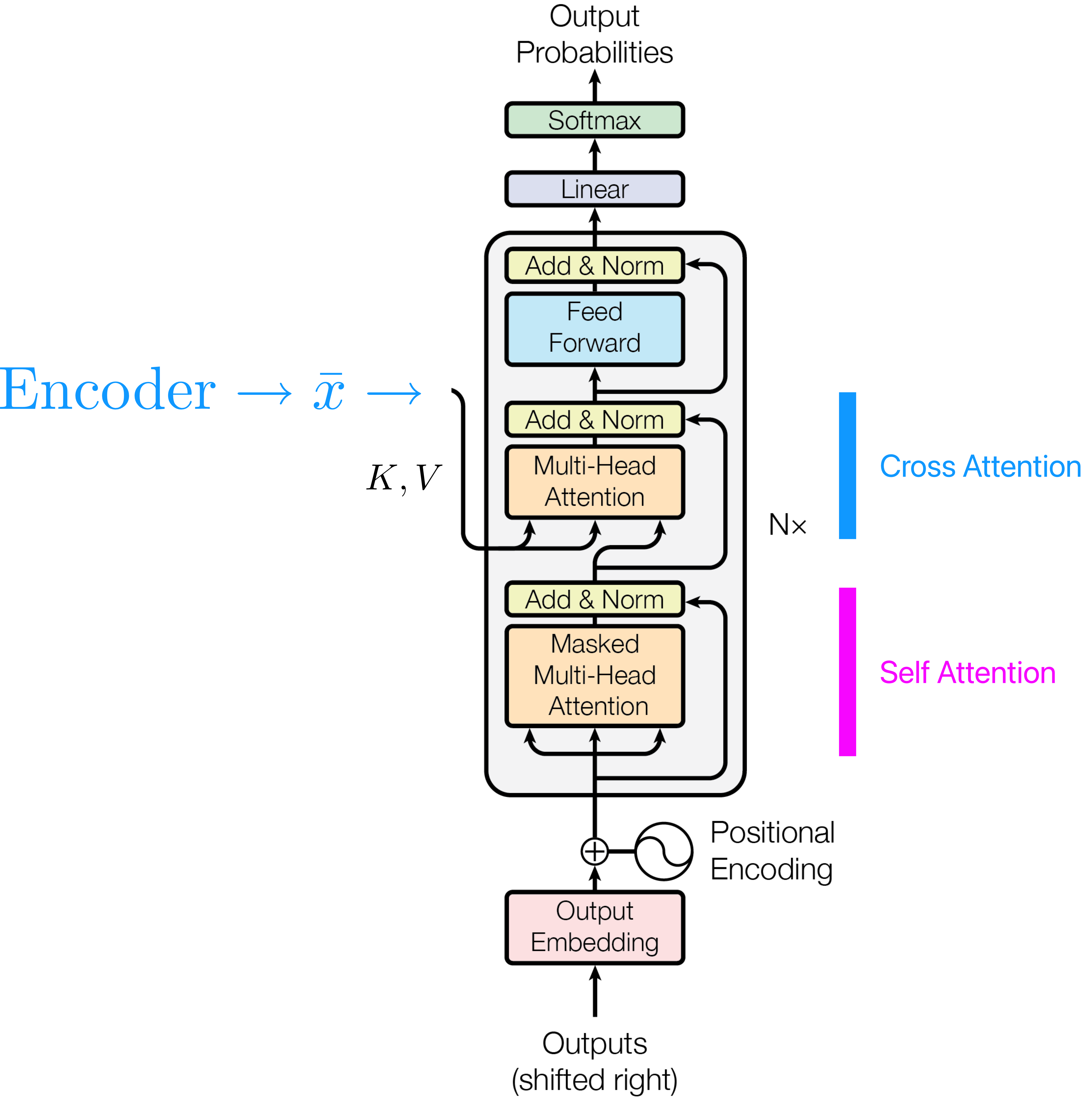
The decoder generates output text sequences step by step.
Components
1. Output Embedding
- Similar to encoder input embedding
- Converts output tokens to vectors
2. Positional Encoding
- Same as encoder
- Tracks position in output sequence
3. Stack of Decoder Layers
The original Transformer uses N = 6 identical decoder layers. Each layer contains:
3.1 Masked Self-Attention Mechanism
- Similar to encoder self-attention but with masking
- Prevents positions from attending to subsequent positions
- Ensures predictions depend only on known outputs at previous positions
- Maintains autoregressive property (can't look into the future)
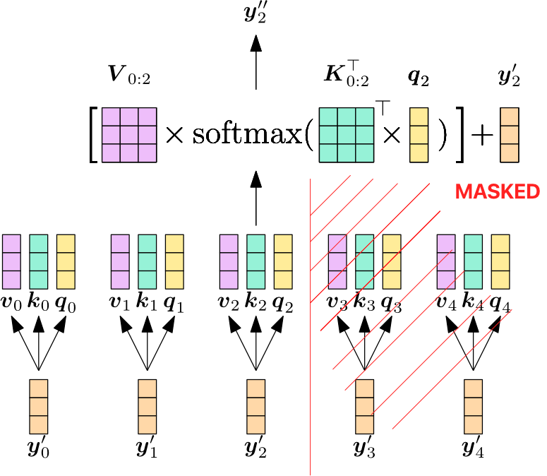
Why masking?
- During training, we have the full target sequence
- But at inference, we generate one token at a time
- Masking simulates the generation process during training
Masked attention is like taking a test where you can only see questions you've already answered, not future questions.
3.2 Encoder-Decoder Multi-Head Attention (Cross Attention)
- Queries (Q): Come from the decoder's previous layer
- Keys (K) and Values (V): Come from the encoder's output
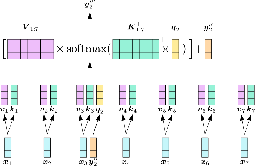
Purpose:
- Aligns decoder's generation with encoded input sequence
- Allows decoder to focus on relevant parts of source input
- Creates connection between input and output sequences
Cross attention is like a translator reading the original text (encoder output) while writing the translation (decoder), constantly referring back to the source.
3.3 Feed-Forward Neural Network
- Similar to encoder's feed-forward network
- Two linear layers with ReLU activation
- Applied separately and identically to each position
- Followed by residual connection and normalization
Normalization and Residual Connections:
- Each sub-layer includes:
- Layer normalization
- Residual connection
- Helps with gradient flow and training stability
4. Linear Classifier and Softmax
- Final step of decoder
- Linear layer: Acts as classifier over vocabulary
- Softmax layer: Converts scores to probabilities
Formula:
- Highest probability indicates predicted next word
- Process continues until end token is generated
Autoregressive Generation
Process:
- Start with special start token (BOS - Beginning Of Sequence)
- Decoder generates first output token
- This token is added to decoder input
- Decoder generates next token
- Repeat until end token (EOS - End Of Sequence) is generated
Key property:
- Each step uses:
- All previously generated tokens
- Full encoder output (with cross attention)
- But cannot see future tokens (due to masking)
Complete Transformer Workflow
Encoding Phase:
Input: "I want to buy a car EOS"
       ↓
  [Tokenization]
       ↓
  [Embedding + Positional Encoding]
       ↓
  [Encoder Layer 1]
       ↓
  [Encoder Layer 2]
       ↓
       ⋮
       ↓
  [Encoder Layer 6]
       ↓
  Encoded Representation (x̄₁, x̄₂, ..., x̄₇)
Decoding Phase:
Start: BOS token
       ↓
  [Decoder generates using encoded input]
       ↓
  Output: 車 (car)
       ↓
  [Feed back: BOS, 車]
       ↓
  Output: を (particle)
       ↓
  [Feed back: BOS, 車, を]
       ↓
       ⋮
       ↓
  Output: です (polite ending)
       ↓
  Output: EOS (stop)

Final output: "車を買いたいです" (I want to buy a car)
Key Advantages of Transformers
-
Parallelization
- Can process entire sequence simultaneously
- Much faster training than sequential RNNs
- Better GPU utilization
-
Long-Range Dependencies
- Direct connections between any two positions
- No information bottleneck
- Better at capturing long-distance relationships
-
No Vanishing Gradients
- Direct paths for gradient flow
- Each position has constant path length to any other position
- More stable training
-
Interpretability
- Attention weights can be visualized
- Shows what the model focuses on
- Helps understand model decisions
The Transformer is like having a team of experts (attention heads) who can all look at the entire document simultaneously and discuss it together, rather than passing notes one by one (like RNNs).
Summary Comparison
| Feature | RNN | LSTM | Transformer |
|---|---|---|---|
| Architecture | Recurrent | Gated recurrent | Attention-based |
| Sequential Processing | Yes | Yes | No (parallel) |
| Long-term Dependencies | Poor (vanishing gradients) | Good (gates) | Excellent (direct connections) |
| Training Speed | Slow | Slow | Fast |
| Memory Mechanism | Hidden state | Cell state + hidden state | Self-attention |
| Complexity | Low | Medium | High |
| Best For | Short sequences | Medium sequences | Long sequences, translation |
References
• von Platen, Patrick. Transformers-based Encoder-Decoder Models. Hugging Face Blog. https://huggingface.co/blog/encoder-decoder
• Vaswani et al. (2017). Attention is All You Need. NeurIPS.
Additional Notes
Key Takeaways:
-
RNNs introduced the concept of sequential processing with memory but suffer from vanishing gradients
-
LSTMs solved the vanishing gradient problem through:
- Gating mechanisms (forget, input, output gates)
- Cell state with additive updates
- Ability to learn long-term dependencies
-
Transformers revolutionized sequence modeling by:
- Eliminating recurrence entirely
- Using self-attention to capture dependencies
- Enabling parallel processing
- Achieving state-of-the-art results in many tasks
-
Self-attention is the key innovation that allows:
- Each position to attend to all other positions
- Capturing global dependencies efficiently
- Better handling of long-range relationships
Practical Considerations:
- Use RNNs for: Simple sequence tasks, resource-constrained environments
- Use LSTMs for: Time series, speech recognition, moderate-length sequences
- Use Transformers for: NLP tasks, machine translation, long documents, when computational resources are available
Modern deep learning has largely moved toward Transformer architectures for sequence modeling tasks, but understanding RNNs and LSTMs provides crucial foundations for understanding how we got here and when simpler models might still be appropriate.