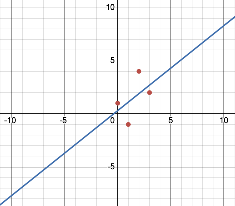
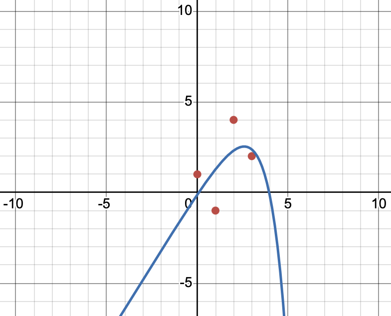
จะคล้าย ๆ กับ 7 – Interpolation แต่ไม่เหมือนเสียทีเดียว เพราะในกรณีนี้เรามีการ “จำกัดรูปแบบของสมการ” ให้เป็นหน้าตาที่กำหนดไว้ล่วงหน้า เช่น อยากให้เป็นสมการกำลังสอง แต่ใน Interpolation จะเลือกสมการที่ “ง่ายที่สุด” ซึ่งสามารถผ่านทุกจุดได้

ต้องทำเป็น

• Solving Least-Squares The Method of Normal Equations
• Solving Least-Squares with QR Factorization
• Householder Transformations
• Givens Rotations

Classic Application: Data Fitting

Example: Fitting a Quadratic Function

• Problem: Fit a quadratic function through five given data points $(t_i, y_i)$, $i = 1, 2, \ldots, 5$
• Unknown quadratic: $y = ct^2 + dt + e$
• Goal: We want the quadratic to pass through all five data points (if possible)

This means we need to satisfy:

Matrix Formulation

This is equivalent to solving:

for $c, d, e$.

• This is a linear system: $\boxed{Ax = b}$
• More rows than columns ⇒ The system is overdetermined
• In general, there is no solution
• That is, no quadratic function that passes through all five data points

Analogy: Imagine trying to draw a smooth parabola (curve) through 5 random dots on paper. Unless the dots happen to lie perfectly on a parabola already, you can't make a single curve pass through all of them exactly!

Alternative Approach: Best Fit

Since we can't find $x$ such that $Ax = b$ exactly:

• How about finding $x$ such that $Ax$ is as close to $b$ as possible?
• That is, find $x$ that minimizes $\|Ax - b\|_2$
  • 3 - Norms, 6 - More on Solving Linear Systems

Analogy: If you can't hit the bullseye exactly, try to get as close as possible!

Linear Least-Squares Problem

Given: $A \in \mathbb{R}^{m \times n}$ and $b \in \mathbb{R}^m$

Find: $x \in \mathbb{R}^n$ that minimizes $\boxed{\|Ax - b\|_2}$

• Sometimes written as $\boxed{Ax \cong b}$

Why Use the 2-Norm?

Reason 1: Computational Ease

• 2-norm problem ($\min \|Ax - b\|_2$): Can be solved using calculus and linear algebra
• 1-norm problem ($\min \|Ax - b\|_1$) and ∞-norm problem ($\min \|Ax - b\|_\infty$): These are linear programming (linear optimization) problems
• 3-norm problem ($\min \|Ax - b\|_3$): This is convex nonlinear programming

The 2-norm is mathematically "smooth" and differentiable, making it much easier to work with analytically.

Reason 2: Statistical Reasons

• The 2-norm (squared) has strong statistical foundations
• Related to maximum likelihood estimation under Gaussian noise assumptions
• Related to minimizing variance in statistical models

Assumptions

Throughout this chapter, we assume:

• $m > n$ (more equations than unknowns - overdetermined system)
• $\text{rank}(A) = n$ (full column rank - columns are linearly independent)

Note: The cases where $\text{rank}(A) < n$ or $m < n$ are more difficult and require different techniques to solve (covered later).

Analogy: We assume we have more data points than parameters to fit (overdetermined), and that all our parameters are actually meaningful and independent (full rank).

Solving Least-Squares: The Method of Normal Equations

วิธีการ Solve แรก

Goal

We want to minimize $\|Ax - b\|_2$

Key Insight

This is the same as minimizing $\|Ax - b\|_2^2$ since $\|Ax - b\|_2 \geq 0$ by definition of norm.

Why square it? Because the square root function is monotonic, the minimum of $f(x)$ occurs at the same point as the minimum of $[f(x)]^2$. Squaring eliminates the square root and makes the math easier!

Mathematical Setup

Recall:

• $\|w\|_2^2 = w^T w$
• $(BC)^T = C^T B^T$

We can expand:

Important observation: $b^T Ax$ is a scalar

• So its transpose equals itself: $(b^T Ax)^T = x^T A^T b = b^T Ax$

Therefore:

Lemma 1: Properties of $A^T A$

Proof:

Part 1 - Symmetry:

• $(A^T A)^T = A^T (A^T)^T = A^T A$ ✓

Part 2 - Positive Definiteness:

• Suppose $x \in \mathbb{R}^n$ is nonzero

• Then:
  $x^T A^T Ax = (Ax)^T Ax = \|Ax\|_2^2 \geq 0$

• But $Ax$ is a nontrivial linear combination of columns of $A$ (since $x \neq 0$)

• Since columns of $A$ are linearly independent (because rank of $A$ is $n$), we have $Ax \neq 0$

• So $\|Ax\|_2 \neq 0$

• Therefore: $x^T A^T Ax = \|Ax\|_2^2 > 0$ ✓

Why this matters: $A^T A$ being symmetric positive definite means it's invertible, which is crucial for finding a unique solution to our least-squares problem!

Lemma 2: Minimizer of Quadratic Forms

Proof:

Step 1: Evaluate $f(x^*)$

First:
$f(x^*) = f(C^{-1}h) = (C^{-1}h)^T CC^{-1}h - 2h^T C^{-1}h + d$
$= h^T C^{-T}h - 2h^T C^{-1}h + d$

But $C$ is symmetric, so:
$C^{-T} = (C^T)^{-1} = C^{-1}$

Therefore:
$f(x^*) = h^T C^{-1}h - 2h^T C^{-1}h + d = -h^T C^{-1}h + d$

Step 2: Evaluate $f(x^* + y)$ for any nonzero vector $y$ (one way to show $x^*$ is unique minimizer)

Let $y \in \mathbb{R}^n$ be any arbitrary nonzero vector.

We have:
$f(x^* + y) = (C^{-1}h + y)^T C(C^{-1}h + y) - 2h^T(C^{-1}h + y) + d$
$= (h^T C^{-1} + y^T)(h + Cy) - 2h^T C^{-1}h - 2h^T y + d$
$= h^T C^{-1}h + h^T C^{-1}Cy + y^T h + y^T Cy - 2h^T C^{-1}h - 2h^T y + d$
$= h^T C^{-1}h + h^T y + y^T h + y^T Cy - 2h^T C^{-1}h - 2h^T y + d$

But $h^T y = \sum_i h_i y_i = y^T h$ (scalars are symmetric).

So:
$f(x^* + y) = h^T C^{-1}h + 2h^T y + y^T Cy - 2h^T C^{-1}h - 2h^T y + d$
$= -h^T C^{-1}h + d + y^T Cy = f(x^*) + y^T Cy$

Step 3: Show $x^*$ is the unique minimizer

But $C$ is symmetric positive definite, so:
$y^T Cy > 0$

Therefore:
$f(x^* + y) = f(x^*) + y^T Cy > f(x^*)$

So $x^*$ is the unique minimizer. ✓

The Solution: Normal Equations

Recall that we want to minimize equation (1):
$\|Ax - b\|_2^2 = x^T A^T Ax - 2b^T Ax + b^T b$

Compare this with Lemma 2:
$f(x) = x^T Cx - 2h^T x + d$

Setting:

• $C = A^T A$
• $h = A^T b$
• $d = b^T b$

We have that $\|Ax - b\|_2^2$ is minimized at:
$\boxed{x^* = C^{-1}h = (A^T A)^{-1}A^T b}$

Main Theorem

Method of Normal Equations

To solve $\min_x \|Ax - b\|_2$:

1. Form products $A^T A$ and $A^T b$
2. Solve แ using Cholesky factorization
   • (Assuming $\text{rank}(A) = n$, Lemma 1 tells us that $A^T A$ is symmetric positive definite)

The equation $\boxed{A^T Ax = A^T b}$ is called the normal equations.

• ไม่ควรใช้ GEPP เนอะ
• $\text{rank}(A) = n$ ถึงจะใช้ Method ที่ว่ามาได้

Example 1: Fitting a Line

(2)
Problem: Given data points $(x, y)$: $(0, 1), (1, -1), (2, 4), (3, 2)$. We want to fit these 4 points with the line $y = mx + c$. Find the line that best fits the data points in least-squares sense using the method of normal equations.

Solution:

We want $m$ and $c$ satisfying:
$mx_1 + c \cong y_1$
$mx_2 + c \cong y_2$
$mx_3 + c \cong y_3$
$mx_4 + c \cong y_4$
In matrix form:
$\begin{bmatrix} x_1 & 1 \\ x_2 & 1 \\ x_3 & 1 \\ x_4 & 1 \end{bmatrix} \begin{bmatrix} m \\ c \end{bmatrix} \cong \begin{bmatrix} y_1 \\ y_2 \\ y_3 \\ y_4 \end{bmatrix}$

Substituting the data points:
$\begin{bmatrix} 0 & 1 \\ 1 & 1 \\ 2 & 1 \\ 3 & 1 \end{bmatrix} \begin{bmatrix} m \\ c \end{bmatrix} \cong \begin{bmatrix} 1 \\ -1 \\ 4 \\ 2 \end{bmatrix}$

Let's call the matrix $A$ and the right-hand side vector $b$.

By the method of normal equations:

$A^T A = \begin{bmatrix} 0 & 1 & 2 & 3 \\ 1 & 1 & 1 & 1 \end{bmatrix} \begin{bmatrix} 0 & 1 \\ 1 & 1 \\ 2 & 1 \\ 3 & 1 \end{bmatrix} = \begin{bmatrix} 14 & 6 \\ 6 & 4 \end{bmatrix}$

5555 คือเนื่องจากมันเป็น Symmetric เนอะ ไม่ต้อง Compute ทั้งหมด ก็ก็อบมาจากข้างบนเลย

And:
$A^T b = \begin{bmatrix} 0 & 1 & 2 & 3 \\ 1 & 1 & 1 & 1 \end{bmatrix} \begin{bmatrix} 1 \\ -1 \\ 4 \\ 2 \end{bmatrix} = \begin{bmatrix} 13 \\ 6 \end{bmatrix}$

Solve $A^T Ax = A^T b$ by Cholesky factorization:
$\begin{bmatrix} 14 & 6 \\ 6 & 4 \end{bmatrix} \begin{bmatrix} m \\ c \end{bmatrix} = \begin{bmatrix} 13 \\ 6 \end{bmatrix}$

The solution is $m = 0.8$, $c = 0.3$.

So the best-fit line in least-squares sense is:
$\boxed{y = 0.8x + 0.3}$

📄 CSS322_Doable_L10_Ex1.pdf

Example 2: Fitting an Exponential Function

Problem: Fit the same data points $(0, 1), (1, -1), (2, 4), (3, 2)$ with the function $y = c_1 x + c_2 e^x$ in least-squares sense using the method of normal equations.

Solution:

We want $c_1$ and $c_2$ satisfying:
$c_1 x_1 + c_2 e^{x_1} \cong y_1$
$c_1 x_2 + c_2 e^{x_2} \cong y_2$
$c_1 x_3 + c_2 e^{x_3} \cong y_3$
$c_1 x_4 + c_2 e^{x_4} \cong y_4$

In matrix form:
$\begin{bmatrix} x_1 & e^{x_1} \\ x_2 & e^{x_2} \\ x_3 & e^{x_3} \\ x_4 & e^{x_4} \end{bmatrix} \begin{bmatrix} c_1 \\ c_2 \end{bmatrix} \cong \begin{bmatrix} y_1 \\ y_2 \\ y_3 \\ y_4 \end{bmatrix}$

Substituting the data points:
$\begin{bmatrix} 0 & e^0 \\ 1 & e^1 \\ 2 & e^2 \\ 3 & e^3 \end{bmatrix} \begin{bmatrix} c_1 \\ c_2 \end{bmatrix} \cong \begin{bmatrix} 1 \\ -1 \\ 4 \\ 2 \end{bmatrix}$

The method of normal equations:
$A^T A = \begin{bmatrix} 14 & 77.7530 \\ 77.7530 & 466.4160 \end{bmatrix}$

And:
$A^T b = \begin{bmatrix} 13 \\ 68.0090 \end{bmatrix}$

Solve $A^T A \begin{bmatrix} c_1 \\ c_2 \end{bmatrix} = A^T b$ by Cholesky factorization.

The solution is $c_1 = 1.6013$, $c_2 = -0.1211$.

So the best-fit function is:
$\boxed{y = 1.6013x - 0.1211e^x}$

Running Time of Method of Normal Equations

Matrix multiplication complexity:

• $A \in \mathbb{R}^{p \times q}$, $B \in \mathbb{R}^{q \times r}$
• Multiplying $AB$ requires $2pqr$ arithmetic operations
• The matrix $C = AB$ is $p$-by-$r$ matrix
• To find $c_{ij} = \sum_{k=1}^q a_{ik} b_{kj}$, need $2q$ operations
• $C$ has $pr$ entries, so $2pqr$ operations total

For normal equations:

• But $A^T A$ is symmetric, so only need to compute the upper triangular portion
• Therefore, Step 1 needs $mn^2 + O(mn)$ operations
• Step 2 requires $n^3/3 + O(n^2)$ operations (running time of Cholesky factorization)

Total arithmetic operations:
$\boxed{mn^2 + n^3/3 + O(mn) = mn^2 + O(n^3 + mn)}$ (assuming $m \geq n$)

Comment on the Method of Normal Equations

Advantages:

• The method of normal equations is fast
• $A^T A$ is smaller than $A$ and is symmetric
• So solving $A^T Ax = A^T b$ is fast

Stability:

• The method is conditionally stable but not backward stable
• This means numerical errors can accumulate in certain ill-conditioned problems

QR Factorization

อีก Method นึง

Structure of $R$:
$R = \begin{bmatrix} R_1 \\ 0 \end{bmatrix}$

where:

• $R_1$ is an $n$-by-$n$ upper triangular matrix
• $0$ is an $(m-n)$-by-$n$ zero matrix

Examples of $R$:
$\begin{bmatrix} 1 & 3 \\ 0 & 2 \\ 0 & 0 \end{bmatrix}, \quad \begin{bmatrix} 4 & 1 & 2 \\ 0 & 2 & 5 \\ 0 & 0 & -1 \\ 0 & 0 & 0 \\ 0 & 0 & 0 \end{bmatrix}$

ก็คือ $R$ มันไม่ใช่ Upper triangular matrix แบบธรรมดานะ มันต้องมี extra row of 0s อยู่ข้างล่างด้วย

Solving Least-Squares with QR Factorization

Suppose we have a QR factorization of $A$:
$A = QR$

We want to minimize:
$\|Ax - b\|_2 = \|QRx - b\|_2$

Key step: Let $c = Q^T b$. That is, $b = Qc$.

So:
$\|Ax - b\|_2 = \|QRx - Qc\|_2$
$= \|Q(Rx - c)\|_2$
$= \|Rx - c\|_2 \quad \text{(since } \|Qx\|_2 = \|x\|_2 \text{ for orthogonal } Q)$
$= \left\|\begin{bmatrix} R_1 \\ 0 \end{bmatrix} x - \begin{bmatrix} c_1 \\ c_2 \end{bmatrix}\right\|_2$

where $c = \begin{bmatrix} c_1 \\ c_2 \end{bmatrix}$, $c_1 \in \mathbb{R}^n$, and $c_2 \in \mathbb{R}^{m-n}$.

Simplifying:
$\|Ax - b\|_2 = \left\|\begin{bmatrix} R_1 x - c_1 \\ -c_2 \end{bmatrix}\right\|_2 = \sqrt{\|R_1 x - c_1\|_2^2 + \|c_2\|_2^2}$

Key observation: $c_2$ is a constant (it does not depend on $x$ since $c = Q^T b$).

So the $x$ that minimizes $\|Ax - b\|_2$ is the one that minimizes $\|R_1 x - c_1\|_2$.

If $R_1$ is nonsingular, then:
$R_1 x = c_1$

has a solution. This solution $x$ satisfies:
$R_1 x - c_1 = 0$
$\|R_1 x - c_1\|_2 = 0$

In other words, this solution $x$ minimizes $\|R_1 x - c_1\|_2$ and therefore minimizes $\|Ax - b\|_2$.

Theorems for QR Factorization

Conclusion: If $\text{rank}(A) = n$, the least-squares problem can always be solved using QR factorization.

Algorithm: Solving Least-Squares with QR Factorization

Steps to solve $\min_x \|Ax - b\|_2$:

1. Factor $A = QR$
2. Compute $c = Q^T b$
3. Solve $R_1 x = c_1$ for $x$ by back substitution
   • Backward stable and fast than GEPP อีกนะ เลยใช้เลยล่ะ

Example 3: Using QR Factorization

Problem: Solve the least-squares problem:
$\begin{bmatrix} 1 & 2 \\ 0 & -2.4 \\ 0 & 1.8 \end{bmatrix} x \cong \begin{bmatrix} -1 \\ 0 \\ 1 \end{bmatrix}$

Given QR factorization:
$\begin{bmatrix} 1 & 2 \\ 0 & -2.4 \\ 0 & 1.8 \end{bmatrix} = \begin{bmatrix} 1 & 0 & 0 \\ 0 & 0.8 & 0.6 \\ 0 & -0.6 & 0.8 \end{bmatrix} \begin{bmatrix} 1 & 2 \\ 0 & -3 \\ 0 & 0 \end{bmatrix}$

Solution:

Step 1: Let
$c = Q^T b = \begin{bmatrix} 1 & 0 & 0 \\ 0 & 0.8 & -0.6 \\ 0 & 0.6 & 0.8 \end{bmatrix} \begin{bmatrix} -1 \\ 0 \\ 1 \end{bmatrix} = \begin{bmatrix} -1 \\ -0.6 \\ 0.8 \end{bmatrix}$

Step 2: Since $A$ is 3-by-2:
$c_1 = \begin{bmatrix} -1 \\ -0.6 \end{bmatrix}$

Step 3: Solve $R_1 x = c_1$:
$\begin{bmatrix} 1 & 2 \\ 0 & -3 \end{bmatrix} x = \begin{bmatrix} -1 \\ -0.6 \end{bmatrix}$

by back substitution.

The solution is:
$\boxed{x = \begin{bmatrix} -1.4 \\ 0.2 \end{bmatrix}}$
which is also the solution to the least squares problem.
📄 CSS322_Doable_L10_Ex3.pdf

Summary

Two main methods for solving least-squares problems:

Method 1: Normal Equations

• Solve: $A^T A x = A^T b$
• Advantages: Fast, simple
• Disadvantages: Conditionally stable (can have numerical issues)
• Running time: $mn^2 + O(n^3 + mn)$

Method 2: QR Factorization

• Solve: Factor $A = QR$, then solve $R_1 x = c_1$ where $c_1$ are top $n$ entries of $Q^T b$
• Advantages: More numerically stable, backward stable
• Disadvantages: Slower than normal equations
• Running time: $2mn^2 - \frac{2n^3}{3} + O(mn)$

When to use which?

• Use normal equations when speed is critical and $A$ is well-conditioned
• Use QR factorization when numerical stability is important or $A$ is ill-conditioned

QR Factorization Algorithms

Three main algorithms for computing QR factorization:

1. Householder transformations (most commonly used)
2. Givens rotations (useful for sparse matrices)
3. Gram-Schmidt algorithm (simple but less stable)

Householder Transformations

Definition

Let $v \in \mathbb{R}^m$ be a nonzero vector. $\boxed{H = I - 2\frac{vv^T}{v^T v}}$

is called a Householder transform/reflection/matrix.

Proof of Properties

Part 1 - Symmetry: (เวลาโชว์ทำไงนะ ก็โชว์ว่า $H^T = H$ ไง)

$H^T = \left(I - 2\frac{vv^T}{v^T v}\right)^T = I^T - 2\frac{(vv^T)^T}{v^T v} = I - 2\frac{vv^T}{v^T v} = H$

Part 2 - Orthogonality: (นี่ล่ะ $HH^T=I$)

$HH^T = HH = \left(I - 2\frac{vv^T}{v^T v}\right)\left(I - 2\frac{vv^T}{v^T v}\right)$

$= I - 4\frac{vv^T}{v^T v} + 4\frac{vv^T vv^T}{(v^T v)^2}$

$= I - 4\frac{vv^T}{v^T v} + 4\frac{v(v^T v)v^T}{(v^T v)^2}$

$= I - 4\frac{vv^T}{v^T v} + 4\frac{vv^T}{v^T v} = I$

Using Householder to Create Zeros

Goal: Given a vector $a$ (say, the first column of $A$), we want a Householder transform such that:

$Ha = \left(I - 2\frac{vv^T}{v^T v}\right)a = \begin{bmatrix} \alpha \\ 0 \\ \vdots \\ 0 \end{bmatrix} = \alpha e_1$

for some scalar $\alpha$ (which will be the first column of $R$).

Solution: This is satisfied by taking:

• $v := a - \alpha e_1$
• $\alpha = \pm \|a\|_2$

To avoid cancellation: Choose $\alpha$ to have the opposite sign from $a_1$: $\boxed{\alpha = -\text{sign}(a_1) \|a\|_2}$

This ensures numerical stability by avoiding subtraction of nearly equal numbers.

Verification

We need to verify that $Ha = \alpha e_1$.

Starting with:
$Ha = \left(I - 2\frac{vv^T}{v^T v}\right)a = a - 2\frac{vv^T}{v^T v}a$

After substituting $v = a - \alpha e_1$ and simplifying (detailed algebra in the slides):

$Ha = \alpha e_1$ ✓

Algorithm: QR Factorization via Householder

Given: $A \in \mathbb{R}^{m \times n}$

Process:

1. Write $A = [a \quad B]$ where $a \in \mathbb{R}^m$ is the first column
2. Choose $H_1$ to annihilate first column:
   • Set $v_1 := a - \alpha_1 e_1$ where $\alpha_1 = -\text{sign}(a_1) \|a\|_2$
   • Then $H_1 = I - 2\frac{v_1 v_1^T}{v_1^T v_1}$
3. After applying $H_1$:
   $H_1 A = \begin{bmatrix} \alpha_1 & w^T \\ 0 & A_2 \end{bmatrix}$
4. Recursively apply to submatrix $A_2$
5. Continue until upper triangular

Result: After $n$ steps: $H_n H_{n-1} \cdots H_1 A = R$

Since $H_i$ are orthogonal and symmetric ($H_i^T = H_i$ and $H_i^T H_i = I$):
$A = H_1 H_2 \cdots H_n R = QR$

where $Q = H_1 H_2 \cdots H_n$ is orthogonal.

Efficient Implementation

Key Optimization 1: Don't Form Q Explicitly

For solving least-squares, we only need $c = Q^T b$:

$c = Q^T b = H_n H_{n-1} \cdots H_2 H_1 b$

Solution: Apply $H_1$ to $b$, then $H_2$ to result, and so on.

Key Optimization 2: Work with Submatrices

For $k > 1$:
$H_k = \begin{bmatrix} I_{k-1} & 0 \\ 0 & H_k' \end{bmatrix}$

This means:
$H_k w = \begin{bmatrix} I_{k-1} & 0 \\ 0 & H_k' \end{bmatrix} \begin{bmatrix} w_1 \\ w_2 \end{bmatrix} = \begin{bmatrix} w_1 \\ H_k' w_2 \end{bmatrix}$

Benefit: Only apply $H_k'$ to relevant portion of vector!

Key Optimization 3: Efficient Multiplication

Computing $Hu$ directly from definition:
$Hu = \left(I - 2\frac{vv^T}{v^T v}\right)u = u - \left(2\frac{v^T u}{v^T v}\right)v$

• This is $O(m)$ operations
• Much cheaper than forming $H$ explicitly and multiplying ($O(m^2)$ operations)

Similarly, for matrix $A$:
$HA = H[a_{\bullet 1} \quad a_{\bullet 2} \quad \cdots \quad a_{\bullet n}] = [Ha_{\bullet 1} \quad Ha_{\bullet 2} \quad \cdots \quad Ha_{\bullet n}]$

Apply the efficient formula to each column.

Example 4: Complete Householder QR Solution

Problem: Use Householder QR factorization to solve:

$\begin{bmatrix} 1 & 5 & 3 \\ 2 & -1 & 3 \\ -2 & 2 & 1 \\ 2 & 0 & 3 \end{bmatrix} x \cong \begin{bmatrix} 2 \\ 0 \\ 1 \\ 0 \end{bmatrix}$

Solution:

Step 1: Annihilate first column

Set $a = \begin{bmatrix} 1 \\ 2 \\ -2 \\ 2 \end{bmatrix}$ (first column of $A$)

Since $a_1 = 1 > 0$, set:
$\alpha = -\|a\|_2 = -3.6056$

$v_1 = a - \alpha e_1 = \begin{bmatrix} 1 \\ 2 \\ -2 \\ 2 \end{bmatrix} - (-3.6056)\begin{bmatrix} 1 \\ 0 \\ 0 \\ 0 \end{bmatrix} = \begin{bmatrix} 4.6056 \\ 2 \\ -2 \\ 2 \end{bmatrix}$

Apply to get: $\boxed{Hu = u - (2\frac{vv^T}{v^T v})v}$

• สำหรับ First Column; $u$ ให้ใช้เป็น first column of $A$ แล้ว $v$ ก็เป็นอันข้างบนที่ได้มา $v_1$
• Second column; คล้าย ๆ กัน แต่ $u$ ก็ใช้เป็น second column of $A$
• …

$H_1 A = \begin{bmatrix} -3.6056 & 0.2774 & -3.6056 \\ 0 & -3.0509 & 0.1315 \\ 0 & 4.0509 & 3.8685 \\ 0 & -2.0509 & 0.1315 \end{bmatrix}$

Step 2: Annihilate second column of submatrix (เอาแค่ส่วนล่างขวามาแค่นั้น)

Remove first row and column to get:
$A_2 = \begin{bmatrix} -3.0509 & 0.1315 \\ 4.0509 & 3.8685 \\ -2.0509 & 0.1315 \end{bmatrix}$

Set $a = \begin{bmatrix} -3.0509 \\ 4.0509 \\ -2.0509 \end{bmatrix}$ (first column of $A_2$)

Since $a_1 < 0$, set $\alpha = \|a\|_2 = 5.4702$

$v_2 = a - \alpha e_1 = \begin{bmatrix} -8.5211 \\ 4.0509 \\ -2.0509 \end{bmatrix}$

Apply $H'_2$ to $A_2$ to get

Apply to get:
$H_2 H_1 A = \begin{bmatrix} -3.6056 & 0.2774 & -3.6056 \\ 0 & 5.4702 & 2.7421 \\ 0 & 0 & 2.6274 \\ 0 & 0 & 0.7598 \end{bmatrix}$

Step 3: Annihilate third column of submatrix

Remove first two rows and columns:
$A_3 = \begin{bmatrix} 2.6274 \\ 0.7598 \end{bmatrix}$

Since first entry > 0, set $\alpha = -\|a\|_2 = -2.7351$

$v_3 = \begin{bmatrix} 5.3625 \\ 0.7598 \end{bmatrix}$

Apply to get:
$H_3 H_2 H_1 A = \begin{bmatrix} -3.6056 & 0.2774 & -3.6056 \\ 0 & 5.4702 & 2.7421 \\ 0 & 0 & -2.7351 \\ 0 & 0 & 0 \end{bmatrix} = R$

Therefore:
$R_1 = \begin{bmatrix} -3.6056 & 0.2774 & -3.6056 \\ 0 & 5.4702 & 2.7421 \\ 0 & 0 & -2.7351 \end{bmatrix}$(Top square portion of $R$)

Step 4: Form $c = Q^T b$

Apply $H_1$ to $b$:
$H_1 b = \begin{bmatrix} 0 \\ -0.8685 \\ 1.8685 \\ -0.8685 \end{bmatrix}$

Apply $H_2$ to second through fourth entries:
$H_2 H_1 b = \begin{bmatrix} 0 \\ 2.1937 \\ 0.4128 \\ -0.1315 \end{bmatrix}$

Apply $H_3$ to third and fourth entries:
$c = H_3 H_2 H_1 b = \begin{bmatrix} 0 \\ 2.1937 \\ -0.36 \\ -0.2410 \end{bmatrix}$

Step 5: Solve $R_1 x = c_1$ by back substitution

$\begin{bmatrix} -3.6056 & 0.2774 & -3.6056 \\ 0 & 5.4702 & 2.7421 \\ 0 & 0 & -2.7351 \end{bmatrix} x = \begin{bmatrix} 0 \\ 2.1937 \\ -0.36 \end{bmatrix}$

Solution:
$\boxed{x = \begin{bmatrix} -0.1058 \\ 0.3351 \\ 0.1316 \end{bmatrix}}$
📄 CSS322_Doable_L10_Ex4.pdf

Properties of Householder Transformations

Running Time Comparison

For solving least-squares problems:

• Householder (HH): $2mn^2 - \frac{2n^3}{3} + O(mn)$
• Normal equations: $mn^2 + \frac{n^3}{3} + O(mn)$

Analysis:

• If $m \approx n$: The two are about equal
• If $m \gg n$: HH is about twice as slow
• But HH is backward stable!

Backward Stability

Householder exactly solves: $\min_x \|(A + E)x - b\|_2$