Chapter 11 - Deep Neural Networks

11.1 Shallow versus Deep Neural Networks

Definitions

• Shallow Neural Network: A multilayer perceptron with 1 or 2 hidden layers
  • ที่เราเรียนมาก่อนหน้านี้อะ Multilayer Perceptrons
• Deep Neural Network: A multilayer perceptron with more than 2 hidden layers

Why Deep Networks?

Universal Approximation Theorem: A feedforward network with a single hidden layer is sufficient to represent any function

However:

• The single layer may be infeasibly large (ใหญ่ใกล้ $\infty$ เลยล่ะ)
• May fail to learn and generalize correctly
• Using deeper models can:
  • Reduce the number of units required
  • Reduce the amount of generalization error

Analogy: Think of building with LEGO blocks. You could build a complex structure using one massive layer of blocks, but it's often more efficient and stable to build it in multiple layers, with each layer adding specific features.

11.2 Vanishing Gradient Problem

What is it?

When training a deep neural network using gradient descent, the gradient may become very small as it is propagated backward to earlier layers.

Example: 4-Layer Network Gradient Calculation

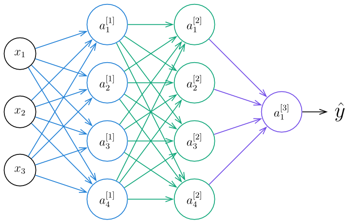
For a network with 4 layers, the gradient is calculated using the chain rule:

$\frac{\partial L}{\partial w^{[3]}_{1,1}} = \left(\frac{\partial L}{\partial \hat{y}}\right) \left(\frac{\partial \hat{y}}{\partial z^{[3]}_1}\right) \left(\frac{\partial z^{[3]}_1}{\partial w^{[3]}_{1,1}}\right)$

$\frac{\partial L}{\partial w^{[2]}_{1,1}} = \left(\frac{\partial L}{\partial \hat{y}}\right) \left(\frac{\partial \hat{y}}{\partial z^{[3]}_1}\right) \left(\frac{\partial z^{[3]}_1}{\partial a^{[2]}_1}\right) \left(\frac{\partial a^{[2]}_1}{\partial z^{[2]}_1}\right) \left(\frac{\partial z^{[2]}_1}{\partial w^{[2]}_{1,1}}\right)$

$\frac{\partial L}{\partial w^{[1]}_{1,1}} = \left(\frac{\partial L}{\partial \hat{y}}\right) \left(\frac{\partial \hat{y}}{\partial z^{[3]}_1}\right) \left(\frac{\partial z^{[3]}_1}{\partial a^{[2]}_1}\right) \left(\frac{\partial a^{[2]}_1}{\partial z^{[2]}_1}\right) \left(\frac{\partial z^{[2]}_1}{\partial a^{[1]}_1}\right) \left(\frac{\partial a^{[1]}_1}{\partial z^{[1]}_1}\right) \left(\frac{\partial z^{[1]}_1}{\partial w^{[1]}_{1,1}}\right)$

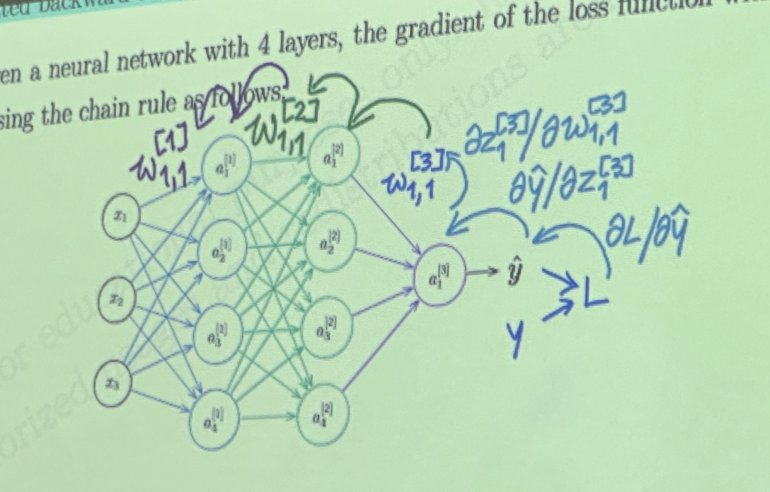
Key Problems:

• Weights farther from the output layer have more terms in the product
• If some terms are less than 1, the overall gradient becomes very small
  • จะต้องมาอัปเดตเนี่ย ถ้า Small Term มาคูณกันก็ยิ่งเล็กเลยล่ะ จนกว่ามันจะ converge เข้า เลขที่ถูกต้องก็ต้องใช้เวลานานไง เพราะสูตรในการ Update จำได้ใช่มั้ย $w_{1,1}^{[1]}\leftarrow w_{1,1}^{[1]}-\eta\frac{\partial L}{\partial w_{1,1}^{[1]}}$
• Weights in earlier layers are not properly updated

Analogy: Like playing telephone with whispers - by the time the message reaches the first person, it's barely audible. Similarly, the gradient signal weakens as it travels back through layers.

11.3 Mitigating Vanishing Gradient

จะทำแก้ปัญหานี้ยังไงล่ะ

Method 1: ReLU Activation Function

ลองเปลี่ยนใช้ ReLU แทนที่จะใช้ Sigmoid บ้างซิ

ReLU (Rectified Linear Unit):
$\boxed{\varphi_{\text{ReLU}}(z) = \max(0, z)}$
$\boxed{\varphi'_{\text{ReLU}}(z) = \begin{cases} 1 & z > 0 \\ 0 & z \leq 0 \end{cases}}$
Benefits:

• Derivative is either 0 or 1
• Prevents gradient from becoming too small
• Commonly used in deep neural networks for hidden layers

Problem: "Dying ReLU"

• Neurons can become inactive and only output zero

Solutions: Leaky ReLU and ELU

Leaky ReLU

$\boxed{\varphi_{\text{leaky}}(z) = \max(0, z) + \alpha \cdot \min(0, z)}$
$\boxed{\varphi'_{\text{leaky}}(z) = \begin{cases} 1 & z > 0 \\ \alpha & z \leq 0 \end{cases}}$

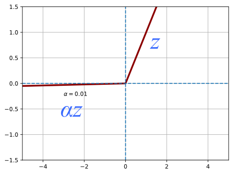
• Typically $\alpha = 0.01$
• Allows small, non-zero gradient when unit is not active

ELU (Exponential Linear Unit)

$\boxed{\varphi_{\text{elu}}(z) = \begin{cases} z & z > 0 \\ \alpha(e^z - 1) & z \leq 0 \end{cases}}$
$\boxed{\varphi'_{\text{elu}}(z) = \begin{cases} 1 & z > 0 \\ \alpha(e^z) & z \leq 0 \end{cases}}$

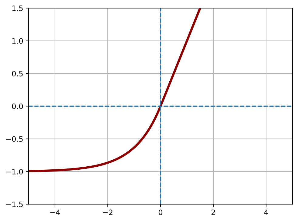
Analogy: ReLU is like a gate that's either fully open (1) or closed (0). Leaky ReLU leaves the gate slightly open even when "closed", allowing a trickle of gradient through.

Method 2: He Initialization

Properly initialize the weight

Purpose: Maintain variance of activations and gradients throughout the network

Formula:

$\boxed{W \sim \mathcal{N}\left(0, \frac{2}{n_{in}}\right)}$

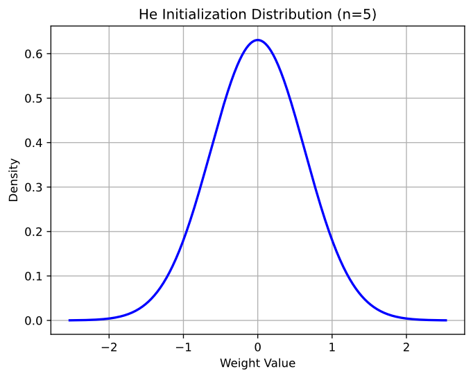
Where $n_{in}$ is the number of input units to the layer

Details:

• Designed for ReLU activation functions
• Weights initialized from normal distribution with:
  • Mean = 0
  • Variance = $\frac{2}{n_{in}}$

Analogy: Like tuning the volume at each stage of an audio system so the signal doesn't get too loud (explode) or too quiet (vanish) as it passes through.

• Makes the gradient become stable, ละช่วยในเรื่อง Vanishing Gradient Problem ได้ดีเลยล่ะ

Method 3: Batch Normalization

Adjust the value in each mini-batch, ปรับค่าใหม่พยายามให้ Mean เป็น 0, Variance เป็น 1

Purpose: Normalize inputs to each layer for each mini-batch, ensuring mean of 0 and variance of 1

Formula:
For each minibatch:
$\mu_B = \frac{1}{B}\sum_{i=1}^{B} x_i\quad \quad \text{(Mean)}$
$\sigma^2_B = \frac{1}{B}\sum_{i=1}^{B} (x_i - \mu_B)^2 \quad \quad \text{(Variance)}$
$\boxed{\hat{x}_i = \frac{x_i - \mu_B}{\sqrt{\sigma^2_B + \epsilon}}}\quad \quad \text{(Standardized value)}$
$\boxed{y_i = \gamma\hat{x}_i + \beta}$

Where:

• $\gamma$ and $\beta$ are learnable parameters → มันจะถูก updated by gradient descent
  • Allow the network to scale ($\gamma$) and shift ($\beta$) the normalized output
• $\epsilon$ is a small constant for numerical stability

Benefits:

• Stabilizes the learning process
• Maintains stable gradients during training

Analogy: Like standardizing test scores across different exams - converting all scores to a common scale (mean 0, variance 1) so they can be fairly compared and processed.

Method 4: Skip Connections (ResNet)

Concept: Allow gradients to flow more directly through the network

Architecture:

x → Layer 1 → Layer 2 → F(x) 
↓                         ↓
└────────────────────────→ + → x + F(x)

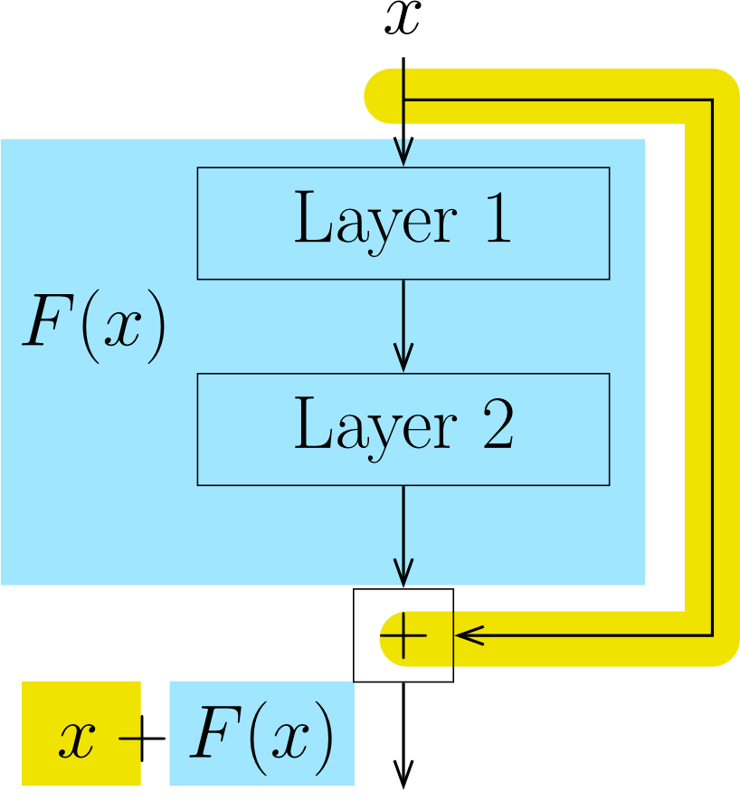
Benefits:

• Reduces likelihood of vanishing gradients in very deep networks
• Creates "shortcuts" for gradient flow

Analogy: Like having express lanes on a highway - traffic (gradients) can bypass congested areas and reach their destination faster.

11.3 Input and Output Encoding

Boolean Attributes

• False = 0
• True = 1

Real-Valued Attributes

Should be normalized or standardized:

Normalization:
$\boxed{z = \frac{x - x_{\min}}{x_{\max} - x_{\min}}}$

• พอเรา Normalize ออกมาจะได้ค่า $\in[0,1]$
  Standardization:
  $\boxed{z = \frac{x - \mu}{\sigma}}$
• หลัง Standardize แล้ว $\mathcal{N}(0,1)$ คือ mean = 0, variance ($\sigma^2$) = 1

When to use:

• Standardization is preferred when values follow a normal distribution
• Helps smooth the optimization landscape
• Speeds up convergence
• If values change enormously among examples, map onto log scale

Analogy: Normalization is like converting temperatures to a 0-1 scale between the coldest and hottest days. Standardization is like expressing temperatures in terms of how many degrees away from average they are.

Categorical Attributes (More than 2 categories)

One-Hot Encoding:
For an attribute with $d$ possible values, use $d$ bits (vector with $d$ elements) where only one bit is 1.

Example: Weather attribute with 4 values: {sun, cloud, rain, snow}

$\text{sun} = \begin{bmatrix} 1 \\ 0 \\ 0 \\ 0 \end{bmatrix}, \quad \text{cloud} = \begin{bmatrix} 0 \\ 1 \\ 0 \\ 0 \end{bmatrix}, \quad \text{rain} = \begin{bmatrix} 0 \\ 0 \\ 1 \\ 0 \end{bmatrix}, \quad \text{snow} = \begin{bmatrix} 0 \\ 0 \\ 0 \\ 1 \end{bmatrix}$

Analogy: Like having separate light switches for each option - only one switch is "on" at a time.

• Put one in different position, to represent different attribute.

Ordinal Attributes

อันนี้คือมันก็เป็น categorical ถูกป้ะ แต่ว่ามันมี Order ของมันด้วย เช่น $\texttt{temperature}\in$ $\{\texttt{low,mid,high}\}$

Ordered Encoding:
For ordered categories where $\text{grp0} < \text{grp1} < \text{grp2} < \text{grp3}$:

$\text{grp0} = \begin{bmatrix} 0 \\ 0 \\ 0 \end{bmatrix}, \quad \text{grp1} = \begin{bmatrix} 1 \\ 0 \\ 0 \end{bmatrix}, \quad \text{grp2} = \begin{bmatrix} 1 \\ 1 \\ 0 \end{bmatrix}, \quad \text{grp3} = \begin{bmatrix} 1 \\ 1 \\ 1 \end{bmatrix}$

Pattern: Cumulative binary representation preserves order

• ถ้าเอาอย่าง $\texttt{temperature}$ ข้างบนก็จะเป็น $\begin{bmatrix} 0 \\ 0\end{bmatrix},\begin{bmatrix} 1 \\ 0\end{bmatrix},\begin{bmatrix} 1 \\ 1\end{bmatrix}$

Analogy: Like filling a measuring cup - each level includes all the previous levels, preserving the ordering.

Example 11.2: Auto MPG Dataset

Objective: Predict fuel efficiency (MPG) from car attributes

Attributes:

1. cylinders:
   • จะมองเป็น Ordinal Value ก็ได้ → $$3=\begin{bmatrix} 0\\0\\0\\0\end{bmatrix},4=\begin{bmatrix} 1\\0\\0\\0\end{bmatrix},5=\begin{bmatrix} 1\\1\\0\\0\end{bmatrix},\dotso$$
   • หรือจะมองเป็น Continuous → ให้ Normalize $z=\frac{x-3}{8-3}$
2. model_year' (transformed ordinal):
   $\text{model\_year}' = \begin{cases} 0 & \text{if model\_year} < 73 \\ 1 & \text{if } 73 \leq \text{model\_year} < 76 \\ 2 & \text{if } 76 \leq \text{model\_year} < 79 \\ 3 & \text{if model\_year} \geq 79 \end{cases}$
   • Use ordered encoding (since it's ordinal)
   $$$$

0=\begin{bmatrix} 0\0\0\end{bmatrix},1=\begin{bmatrix} 1\0\0\end{bmatrix},2=\begin{bmatrix} 1\1\0\end{bmatrix},3=\begin{bmatrix} 1\1\1\end{bmatrix}

\texttt{softmax}(\begin{bmatrix}2\3\1\end{bmatrix})