17 - Partial Differential Equations

เป็น $\partial$ มาให้ แล้วต้องการ $u$
Numerical method for solving Partial Differential Equations (PDE)

Notations

• $u_t = \frac{\partial u}{\partial t}$ - partial derivative with respect to time
• $u_{xy} = \frac{\partial}{\partial y}\left(\frac{\partial u}{\partial x}\right)$ - second-order mixed partial derivative (x first แล้วค่อย y)

Analogy: Think of $u_t$ as measuring how fast something changes over time, and $u_{xy}$ as measuring how the rate of change in the $x$ direction varies as you move in the $y$ direction.

Important PDEs in Practical Applications

Heat Equation

$\boxed{u_t = u_{xx}}$

• Describes heat diffusion in one spatial dimension
• Models how temperature spreads through a material over time

Wave Equation

$\boxed{u_{tt} = u_{xx}}$

• Describes wave propagation in one spatial dimension
• Models vibrations, sound waves, or string oscillations

Laplace Equation

$\boxed{u_{xx} + u_{yy} = 0}$

• Describes steady-state phenomena in two spatial dimensions
• Models equilibrium temperature distribution, electric potential, etc.

Important Note: Many second-order linear PDEs can be transformed into one of the above three equations (plus terms of lower order).

The Heat Equation (Detailed)

General Form

The heat equation in one space dimension:
$\boxed{u_t = cu_{xx}, \quad 0 \leq x \leq L, \quad t \geq 0}$
where $c$ is a positive constant.

$t$ คือเวลานะ, $x$ คือ position

Initial Condition

$u(0, x) = f(x), \quad 0 \leq x \leq L$

• Specifies the initial temperature distribution at time $t = 0$

Boundary Conditions

$u(t, 0) = \alpha, \quad u(t, L) = \beta, \quad t \geq 0$

• Specifies the temperature at both ends of the domain for all time

ให้มาทั้ง Initial condition + Boundary condition เลย5555

Physical Example

• Models the diffusion of heat in a bar of length $L$
• The ends are maintained at temperatures $\alpha$ and $\beta$
• The initial temperature distribution is given by $f(x)$

Analogy: Imagine a metal rod where you heat one end and cool the other. The heat equation tells you how the temperature at each point along the rod changes over time, eventually reaching a steady state.

Initial-Boundary Value Problem for PDE in One Space Dimension

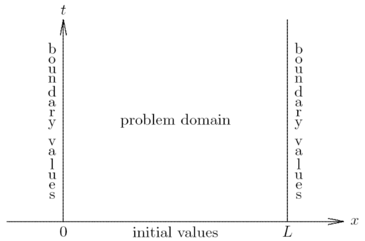
Problem Domain Visualization

• Horizontal axis ($x$): Space from $0$ to $L$
• Vertical axis ($t$): Time from $0$ upward
• Bottom edge: Initial values (at $t = 0$)
• Left edge: Boundary values at $x = 0$
• Right edge: Boundary values at $x = L$
• Interior region: Problem domain where solution must be found

Analogy: Think of this as a rectangular plot where the bottom row shows the starting condition, and the left and right columns show what's happening at the boundaries. You need to fill in all the interior points.

The Wave Equation (Detailed)

General Form

The wave equation in one space dimension:
$\boxed{u_{tt} = cu_{xx}, \quad 0 \leq x \leq L, \quad t \geq 0}$
where $c$ is a positive constant.

Initial Conditions

$u(0, x) = f(x), \quad u_t(0, x) = g(x), \quad 0 \leq x \leq L$

• $f(x)$: initial position/profile
• $g(x)$: initial velocity

Boundary Conditions

$u(t, 0) = \alpha, \quad u(t, L) = \beta, \quad t \geq 0$

Physical Example

• Models vibrations of a violin string of length $L$
• Initial profile given by $f(x)$
• Initial velocity given by $g(x)$
• Ends are anchored (fixed) by the boundary conditions

Analogy: Picture a guitar string. $f(x)$ is how you pull it initially, and $g(x)$ is how fast different parts are moving when you release it. The wave equation predicts how the string will vibrate over time.

The Laplace Equation

Method ในการ solve
We don’t have time ($t$) anymore, but we have 2D space $(x,y)$

General Form

The Laplace equation in two space dimensions:
$\boxed{u_{xx} + u_{yy} = 0}$

• Boundary conditions can be defined in many different ways
• Often used for steady-state problems (no time dependence)

Analogy: Think of a rubber membrane stretched over a frame. The Laplace equation describes the equilibrium shape of the membrane, where it's not moving anymore.

Time-Dependent Problems

Definition

• Time-dependent PDEs: PDEs that have derivatives with respect to $t$ and come with initial conditions
• Examples: Heat equation, Wave equation

Not time-dependent: Laplace equation (no $t$ derivative, no initial conditions)

Numerical Methods for PDEs

Semidiscrete Methods

Work only for time dependent PDE

Main Idea

• Discretize in space only
• Leave time variable continuous
• Converts PDE into a system of ODEs

Example: Heat Equation

Consider the simplified heat equation:

$u_t = cu_{xx}, \quad 0 \leq x \leq 1, \quad t \geq 0$

Initial condition:
$u(0, x) = f(x), \quad 0 \leq x \leq 1$

Boundary conditions:
$u(t, 0) = 0, \quad u(t, 1) = 0, \quad t \geq 0$

Discretization Process

น่าจะเหมือนแปลงให้กลายเป็น $y’_i(t)$ ก็คือ IVP นั่นเอง แล้วค่อยให้อันนั้นแปลงต่อ

1. Introduce spatial mesh points: $x_i = i\Delta x$ for $i = 0, \ldots, n+1$

   • Where $\Delta x = \frac{1}{n+1}$

2. Replace $u_{xx}$ with finite difference approximation:
   $u_{xx}(t, x_i) \approx \frac{u(t, x_{i+1}) - 2u(t, x_i) + u(t, x_{i-1})}{(\Delta x)^2}$

   for $i = 1, \ldots, n$

3. Resulting system of ODEs:
   $\boxed{y_i'(t) = \frac{c}{(\Delta x)^2}(y_{i+1}(t) - 2y_i(t) + y_{i-1}(t))}$

   for $i = 1, \ldots, n$

   where $y_i(t) \approx u(t, x_i)$

4. Boundary conditions: $y_0(t) = y_{n+1}(t) = 0$ for all $t$

5. Initial conditions: $y_i(0) = f(x_i)$ for $i = 1, \ldots, n$

Result: This is an initial value problem for a system of coupled first-order ODEs (RK ก็ได้)

Method of Lines

• Use an ODE solver to solve the initial value problem for this system
• This approach is known as the method of lines
• The resulting ODEs are usually very stiff → choose an appropriate ODE method (e.g., implicit methods)

Analogy: Instead of tracking temperature at every point along the rod (infinite points), we only track it at a finite number of points. The PDE becomes a system of ODEs, one equation for each point showing how its temperature changes based on its neighbors.

Example 1: Method of Lines

Problem Setup

$u_t = 2u_{xx}, \quad 0 \leq x \leq 1, \quad t \geq 0$

Initial condition:
$u(0, x) = \frac{1}{4} - \left(x - \frac{1}{2}\right)^2, \quad 0 \leq x \leq 1$

Boundary conditions:
$u(t, 0) = 0, \quad u(t, 1) = 0, \quad t \geq 0$

Using $n = 3$ interior spatial mesh points.

Solution Steps

1. Calculate $\Delta x$:
   $\Delta x = \frac{1}{3+1} = \frac{1}{4}$

2. Mesh points:

   • $x_0 = 0$, $x_1 = 1/4$, $x_2 = 1/2$, $x_3 = 3/4$, $x_4 = 1$

3. Calculate coefficient:
   $\frac{c}{(\Delta x)^2} = \frac{2}{(1/4)^2} = 32$

4. System of ODEs:
   $y_1'(t) = 32(y_2(t) - 2y_1(t) + y_0(t)) = 32(y_2(t) - 2y_1(t))$
   $y_2'(t) = 32(y_3(t) - 2y_2(t) + y_1(t))$
   $y_3'(t) = 32(y_4(t) - 2y_3(t) + y_2(t)) = 32(-2y_3(t) + y_2(t))$

5. Initial conditions:
   $y_1(0) = \frac{1}{4} - \left(\frac{1}{4} - \frac{1}{2}\right)^2 = \frac{3}{16}$
   $y_2(0) = \frac{1}{4} - \left(\frac{1}{2} - \frac{1}{2}\right)^2 = \frac{1}{4}$
   $y_3(0) = \frac{1}{4} - \left(\frac{3}{4} - \frac{1}{2}\right)^2 = \frac{3}{16}$

6. Vector form:
   $\mathbf{y}'(t) = \begin{bmatrix} y_1'(t) \\ y_2'(t) \\ y_3'(t) \end{bmatrix} = \begin{bmatrix} 32(y_2(t) - 2y_1(t)) \\ 32(y_3(t) - 2y_2(t) + y_1(t)) \\ 32(-2y_3(t) + y_2(t)) \end{bmatrix} = \mathbf{f}(t, \mathbf{y})$
   $\mathbf{y}(0) = \begin{bmatrix} 3/16 \\ 1/4 \\ 3/16 \end{bmatrix}$

Final step: Use an implicit ODE method to solve this initial value problem.

Fully Discrete Methods

Main Idea

• Discretize both space and time variables
  • ตอนนี้ Discretize both $x$ and $t$ นะะ!!
• Replace all derivatives in the PDE by finite difference approximations
• Solve the resulting system of equations

A Fully Discrete Method for the Heat Equation

Problem Setup

$u_t = cu_{xx}, \quad 0 \leq x \leq 1, \quad t \geq 0$

Initial condition:
$u(0, x) = f(x), \quad 0 \leq x \leq 1$

Boundary conditions:
$u(t, 0) = \alpha, \quad u(t, 1) = \beta, \quad t \geq 0$

Discretization

1. Spatial mesh points: $x_i = i\Delta x$ for $i = 0, 1, \ldots, n+1$
   • Where $\Delta x = \frac{1}{n+1}$
2. Temporal mesh points: $t_k = k\Delta t$ for $k = 0, 1, \ldots$
   • Where $\Delta t$ is chosen appropriately
3. Notation: Let $u_i^k$ denote the approximate solution at mesh point $(t_k, x_i)$

Finite Difference Scheme

Replace derivatives with finite differences:

• $u_t$ → forward difference approximation (ฝั่งซ้าย)
• $u_{xx}$ → centered difference approximation (ฝั่งขวา)

For $i = 1, \ldots, n$:

$\frac{u_i^{k+1} - u_i^k}{\Delta t} = c\frac{u_{i+1}^k - 2u_i^k + u_{i-1}^k}{(\Delta x)^2}$

Solving for $u_i^{k+1}$:

$\boxed{u_i^{k+1} = u_i^k + c\frac{\Delta t}{(\Delta x)^2}\left(u_{i+1}^k - 2u_i^k + u_{i-1}^k\right)}$

This is a recurrence relation that can be used iteratively.

Initial and Boundary Conditions

• Initial conditions: $u_i^0 = f(x_i)$ for $i = 1, \ldots, n$
• Boundary conditions: $u_0^k = \alpha$ and $u_{n+1}^k = \beta$ for all $k$

Analogy: Imagine a grid where each point represents temperature at a specific location and time. Starting from the initial temperature distribution (bottom row), you calculate the temperature at each point in the next time step based on its current value and its neighbors' values.

Example 2: Fully Discrete Method

Problem Setup

Same heat equation as Example 1:

$u_t = 2u_{xx}, \quad 0 \leq x \leq 1, \quad t \geq 0$

Initial condition:
$u(0, x) = \frac{1}{4} - \left(x - \frac{1}{2}\right)^2, \quad 0 \leq x \leq 1$

Boundary conditions:
$u(t, 0) = 0, \quad u(t, 1) = 0, \quad t \geq 0$

Using $n = 3$ interior spatial mesh points and $\Delta t = 0.25$.

Solution Steps

1. Same as before: $\Delta x = 1/4$

   • $x_0 = 0$, $x_1 = 1/4$, $x_2 = 1/2$, $x_3 = 3/4$, $x_4 = 1$

2. Initial conditions: $u_1^0 = 3/16$, $u_2^0 = 1/4$, $u_3^0 = 3/16$

3. Boundary conditions: $u_0^0 = 0$, $u_4^0 = 0$

4. First time step ($k = 0 \to 1$):

   Boundary: $u_0^1 = 0$, $u_4^1 = 0$

   Interior points:

   $u_1^1 = u_1^0 + 2\frac{\Delta t}{(\Delta x)^2}(u_2^0 - 2u_1^0 + u_0^0)$
   $= \frac{3}{16} + 2\frac{0.25}{(0.25)^2}\left(\frac{1}{4} - 2\left(\frac{3}{16}\right) + 0\right)$
   $= -0.8125$

   $u_2^1 = u_2^0 + 2\frac{\Delta t}{(\Delta x)^2}(u_3^0 - 2u_2^0 + u_1^0)$
   $= \frac{1}{4} + 2\frac{0.25}{(0.25)^2}\left(\frac{3}{16} - 2\left(\frac{1}{4}\right) + \frac{3}{16}\right)$
   $= -0.75$

   $u_3^1 = u_3^0 + 2\frac{\Delta t}{(\Delta x)^2}(u_4^0 - 2u_3^0 + u_2^0)$
   $= \frac{3}{16} + 2\frac{0.25}{(0.25)^2}\left(0 - 2\left(\frac{3}{16}\right) + \frac{1}{4}\right)$
   $= -0.8125$

5. Continue for subsequent time steps using the same formula...

Warning: Notice the negative values appearing! This suggests the method may be unstable with these parameters. This is a common issue with explicit methods for PDEs.

Properties of the Fully Discrete Method

Accuracy

• Local truncation error: $O(\Delta t) + O((\Delta x)^2)$
  • First-order accurate in time
  • Second-order accurate in space

Scheme Type

• This time-stepping scheme is explicit
• We have a direct formula for obtaining the next point
• No need to solve any equations at each time step

Stability Concerns

• Explicit methods for parabolic PDEs (like heat equation) often have stability restrictions
• Typically require $\Delta t \leq C(\Delta x)^2$ for some constant $C$
• If this condition is violated, the solution may become unstable (oscillate wildly or blow up)

Analogy: An explicit method is like a recipe where you can compute each step directly. An implicit method (not shown here) would require solving a system of equations at each time step, like solving a puzzle, but it's often more stable.

Summary

Key Concepts

1. PDEs vs ODEs: PDEs involve multiple independent variables (space + time), while ODEs involve only one (usually time)

2. Three Important PDEs:

   • Heat equation: diffusion processes
   • Wave equation: oscillatory phenomena
   • Laplace equation: steady-state problems

3. Numerical Approaches:

   • Semidiscrete: Discretize space, keep time continuous → system of ODEs
   • Fully discrete: Discretize both space and time → algebraic equations

4. Method of Lines: Convert PDE to ODE system, then use ODE solvers

5. Explicit vs Implicit:

   • Explicit: Direct computation, but may have stability restrictions
   • Implicit: Requires solving equations, but often more stable

6. Accuracy: Track truncation errors in both space and time separately

Important Formulas

Heat Equation (Explicit Scheme):
$\boxed{u_i^{k+1} = u_i^k + c\frac{\Delta t}{(\Delta x)^2}\left(u_{i+1}^k - 2u_i^k + u_{i-1}^k\right)}$

Centered Difference for Second Derivative:
$\boxed{u_{xx}(t, x_i) \approx \frac{u(t, x_{i+1}) - 2u(t, x_i) + u(t, x_{i-1})}{(\Delta x)^2}}$

Stencil Diagrams

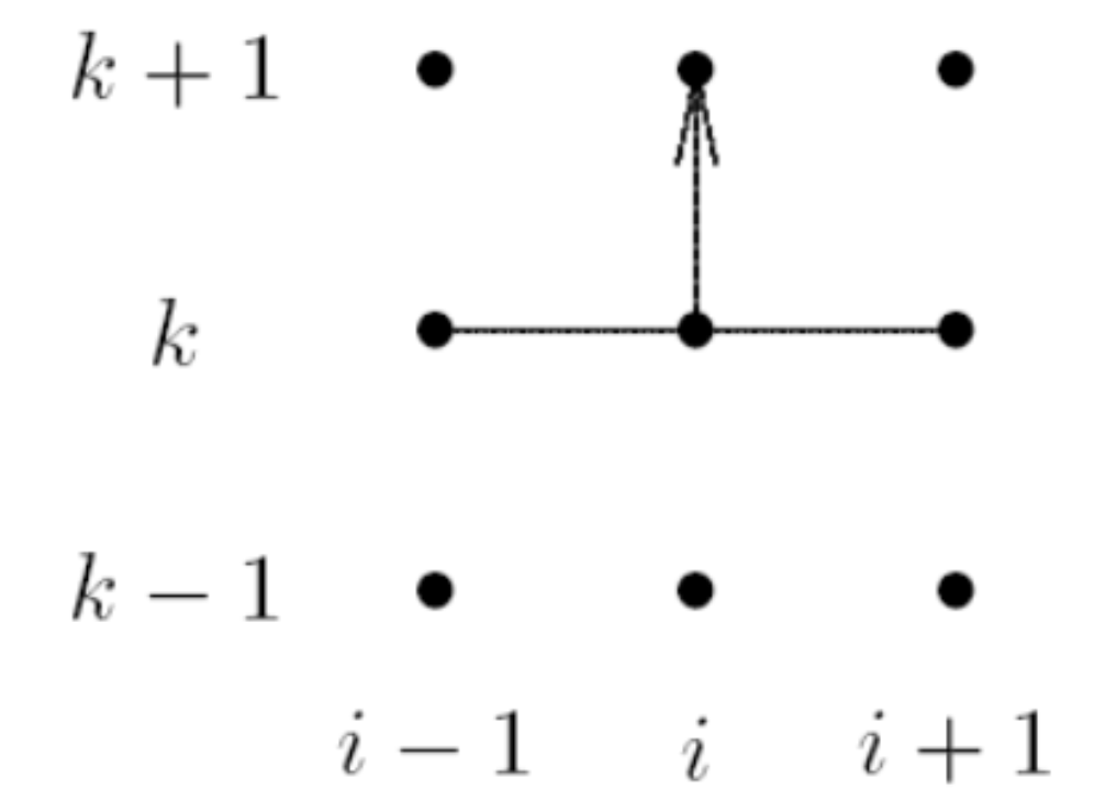
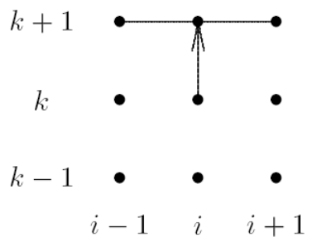
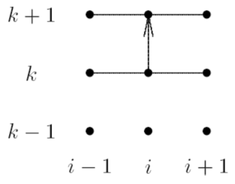
Page 22: Stencil showing the computational pattern for the explicit finite difference scheme for the heat equation.

• Shows three time levels: $k-1$, $k$, and $k+1$
• Shows three spatial points: $i-1$, $i$, and $i+1$
• The point at $(k+1, i)$ depends on three points from time level $k$

Analogy: Think of a stencil as a template showing which neighboring points you need to calculate the next value. Like a cookie cutter pattern - it shows exactly which ingredients (neighboring values) go into making the next cookie (next value).

A Fully Discrete Method for the Wave Equation

Problem Setup

Consider the wave equation:

$u_{tt} = cu_{xx}, \quad 0 \leq x \leq 1, \quad t \geq 0$

Initial conditions:
$u(0, x) = f(x), \quad u_t(0, x) = g(x), \quad 0 \leq x \leq 1$

Boundary conditions:
$u(t, 0) = \alpha, \quad u(t, 1) = \beta, \quad t \geq 0$

Discretization

1. Spatial mesh points: $x_i = i\Delta x$ for $i = 0, 1, \ldots, n+1$

   • Where $\Delta x = \frac{1}{n+1}$

2. Temporal mesh points: $t_k = k\Delta t$ for $k = 0, 1, \ldots$

   • Where $\Delta t$ is chosen appropriately

Finite Difference Scheme

Replace derivatives with centered difference approximations for both $u_{tt}$ and $u_{xx}$.

The PDE becomes (for $i = 1, \ldots, n$):

$\frac{u_i^{k+1} - 2u_i^k + u_i^{k-1}}{(\Delta t)^2} = c\frac{u_{i+1}^k - 2u_i^k + u_{i-1}^k}{(\Delta x)^2}$

Rearranging:

$u_i^{k+1} - 2u_i^k + u_i^{k-1} = c\left(\frac{\Delta t}{\Delta x}\right)^2\left(u_{i+1}^k - 2u_i^k + u_{i-1}^k\right)$

Solving for $u_i^{k+1}$:

$\boxed{u_i^{k+1} = 2u_i^k - u_i^{k-1} + c\left(\frac{\Delta t}{\Delta x}\right)^2\left(u_{i+1}^k - 2u_i^k + u_{i-1}^k\right)}$

Accuracy

• This scheme is second-order accurate in both space and time

Initial Conditions for the Scheme

Challenge: Since we need two previous time levels to compute $u^{k+1}$, we need both $u_i^0$ and $u_i^1$ initially to start.

• คล้าย ๆ Secant Method ที่ต้องการ 2 initial points

Solution from initial conditions:

$u_i^0 = f(x_i), \quad u_i^1 = u_i^0 + \Delta t g(x_i)$

for $i = 1, \ldots, n$.

Note: $u_i^1$ above comes from a forward difference approximation to the initial condition $u_t(0, x) = g(x)$.

• ถ้าไม่เชื่อลองย้ายข้างดู มันเป็น $\frac{u_i^1-u_i^0}{\Delta t}=g(x_i)$

Analogy: The wave equation is like tracking the motion of a vibrating string. You need to know both where the string is initially ($f(x)$) and how fast it's moving ($g(x)$). To start the numerical scheme, you use the initial velocity to estimate where the string will be after the first tiny time step.

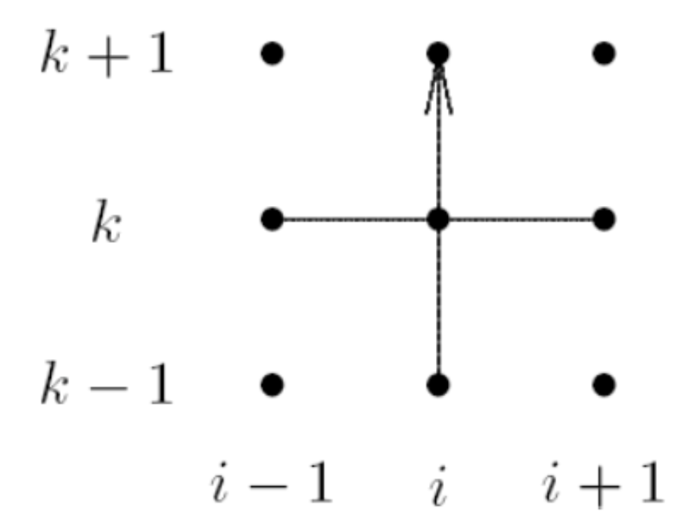
Page 26: Stencil showing the computational pattern for the explicit finite difference scheme for the wave equation.

• Shows three time levels: $k-1$, $k$, and $k+1$
• Shows three spatial points: $i-1$, $i$, and $i+1$
• The point at $(k+1, i)$ depends on five points: three from level $k$ and two from level $k-1$

Example 3: Wave Equation with Fully Discrete Method

Problem Setup

$u_{tt} = 5u_{xx}, \quad 0 \leq x \leq 1, \quad t \geq 0$

Initial conditions:
$u(0, x) = 1 - x, \quad u_t(0, x) = x^2, \quad 0 \leq x \leq 1$

Boundary conditions:
$u(t, 0) = 1, \quad u(t, 1) = 0, \quad t \geq 0$

Using $n = 4$ interior spatial mesh points and $\Delta t = 0.1$.

Solution Steps

1. Calculate $\Delta x$:
   $\Delta x = \frac{1}{n+1} = \frac{1}{4+1} = \frac{1}{5}$

2. Mesh points:
   $x_0 = 0, \quad x_1 = \frac{1}{5}, \quad x_2 = \frac{2}{5}, \quad x_3 = \frac{3}{5}, \quad x_4 = \frac{4}{5}, \quad x_5 = 1$

3. Initial conditions $u_i^0 = f(x_i)$ and $u_i^1 = u_i^0 + \Delta t g(x_i)$:

   $u_1^0 = 1 - x_1 = 1 - \frac{1}{5} = \frac{4}{5}$
   $u_2^0 = 1 - x_2 = 1 - \frac{2}{5} = \frac{3}{5}$
   $u_3^0 = 1 - x_3 = 1 - \frac{3}{5} = \frac{2}{5}$
   $u_4^0 = 1 - x_4 = 1 - \frac{4}{5} = \frac{1}{5}$

4. First time level using initial velocity:

   $u_1^1 = u_1^0 + \Delta t g(x_1) = \frac{4}{5} + (0.1)\left(\frac{1}{5}\right)^2 = 0.804$
   $u_2^1 = u_2^0 + \Delta t g(x_2) = \frac{3}{5} + (0.1)\left(\frac{2}{5}\right)^2 = 0.616$
   $u_3^1 = u_3^0 + \Delta t g(x_3) = \frac{2}{5} + (0.1)\left(\frac{3}{5}\right)^2 = 0.436$
   $u_4^1 = u_4^0 + \Delta t g(x_4) = \frac{1}{5} + (0.1)\left(\frac{4}{5}\right)^2 = 0.264$

5. Boundary conditions:
   $u_0^0 = u_0^1 = 1$
   $u_5^0 = u_5^1 = 0$

6. Second time step ($t = t_2 = 2(\Delta t) = 0.2$):

   First, boundary conditions:
   $u_0^2 = 1, \quad u_5^2 = 0$

   Calculate coefficient:
   $c\left(\frac{\Delta t}{\Delta x}\right)^2 = 5\left(\frac{0.1}{0.2}\right)^2 = 1.25$

   Note: The calculation seems to have an error in the PDF. It should be:
   $c\left(\frac{\Delta t}{\Delta x}\right)^2 = 5\left(\frac{0.1}{1/5}\right)^2 = 5\left(\frac{0.1}{0.2}\right)^2 = 5(0.5)^2 = 1.25$

7. Interior points:

$u_1^2 = 2u_1^1 - u_1^0 + (1.25)(u_2^1 - 2u_1^1 + u_0^1)$
$= 2(0.804) - \frac{4}{5} + (1.25)(0.616 - 2(0.804) + 1) = 0.818$
$u_2^2 = 2u_2^1 - u_2^0 + (1.25)(u_3^1 - 2u_2^1 + u_1^1)$
$= 2(0.616) - \frac{3}{5} + (1.25)(0.436 - 2(0.616) + 0.804) = 0.642$
$u_3^2 = 2u_3^1 - u_3^0 + (1.25)(u_4^1 - 2u_3^1 + u_2^1)$
$= 2(0.436) - \frac{2}{5} + (1.25)(0.264 - 2(0.436) + 0.616) = 0.482$
u_4^2 = 2u_4^1 - u_4^0 + (1.25)(u_5^1 - 2u_4^1 + u_3^1)$$$$= 2(0.264) - \frac{1}{5} + (1.25)(0 - 2(0.264) + 0.436) = 0.213
8. Continue for subsequent time steps using the same formula.

Comparison: Semidiscrete vs Fully Discrete Methods

Semidiscrete Methods

• Even in semidiscrete methods, the time variable is ultimately discretized anyway by the ODE solver
• The difference: we let the (possibly sophisticated) ODE solver choose appropriate step sizes that maintain stability and achieve desired accuracy
• The solver may even change step sizes as needed (adaptive time stepping)

Fully Discrete Methods

• The user must choose time step sizes explicitly
• More direct control but requires more knowledge of stability constraints
• Can be simpler to implement for basic problems

Connection to ODE Methods

• Important observation: The fully discrete method for the heat equation is exactly Euler's method applied to equation (1) (the semidiscrete system of ODEs for the heat equation).

Stability Analysis for Heat Equation

Stability Condition for Explicit Scheme

By stability analysis, the explicit finite difference scheme for the heat equation requires:

$\boxed{\Delta t \leq \frac{(\Delta x)^2}{2c}}$

for the scheme to be stable.

Analogy: This stability condition is like a speed limit. If you try to take too large a time step (go too fast) relative to your spatial grid spacing, the numerical solution will become unstable and blow up - like a car losing control at high speed on a bumpy road.

Important notes:

• As $\Delta x$ decreases (finer spatial mesh), $\Delta t$ must decrease even faster (quadratically)
• This can make explicit methods computationally expensive for fine grids
• This motivates the use of implicit methods

Implicit Methods for the Heat Equation

Backward Euler Method

Applying the backward Euler method to equation (1) yields the implicit finite difference scheme:

$\boxed{u_i^{k+1} = u_i^k + c\frac{\Delta t}{(\Delta x)^2}\left(u_{i+1}^{k+1} - 2u_i^{k+1} + u_{i-1}^{k+1}\right)}$

for $i = 1, \ldots, n$.

Properties:

• Unconditionally stable (no restriction on $\Delta t$)
• Still only first-order accurate in time
• Requires solving a linear system at each time step

Page 35: Stencil showing the backward Euler method applied to the heat equation.

• Shows points at time levels $k$ and $k+1$
• The point at $(k+1, i)$ depends on three points from level $k+1$ (horizontal line)
• Implicit nature: need to solve for all points at level $k+1$ simultaneously

Crank-Nicolson Method

Applying the implicit trapezoid method to equation (1) yields the Crank-Nicolson method:

$\boxed{u_i^{k+1} = u_i^k + c\frac{\Delta t}{(\Delta x)^2}\left(u_{i+1}^{k+1} - 2u_i^{k+1} + u_{i-1}^{k+1} + u_{i+1}^k - 2u_i^k + u_{i-1}^k\right)}$

Properties:

• Unconditionally stable
• Second-order accurate in time (and in space)
• Best overall accuracy among the methods discussed
• Requires solving a linear system at each time step

Computational Efficiency

For both backward Euler and Crank-Nicolson methods for the heat equation in one space dimension:

• The linear system to be solved at each step is tridiagonal
• Tridiagonal systems can be solved very efficiently in $O(n)$ time
• Therefore, these implicit methods are practical despite requiring system solves

Analogy: The Crank-Nicolson method is like averaging your estimate of tomorrow's temperature using both today's data and tomorrow's data. It's more accurate because it "looks both backward and forward" in time, unlike explicit methods that only look backward.

Page 37: Stencil showing the Crank-Nicolson method.

• Shows points at time levels $k-1$, $k$, and $k+1$
• The point at $(k+1, i)$ depends on six points: three from level $k+1$ and three from level $k$
• Symmetric pattern reflecting the averaging nature of the method

Time-Independent Problems

Key Differences from Time-Dependent Problems

• Similar to ODE BVPs, the solution to time-independent PDEs depends on all of the boundary conditions
• The approximate solution must be computed everywhere simultaneously
• Cannot use step-by-step marching as in time-dependent PDEs
• Results in solving a large system of equations

Analogy: Time-independent problems are like solving a jigsaw puzzle where every piece affects every other piece. You can't just build from left to right - you need to consider all the boundary constraints and fit everything together at once.

Finite Difference Methods for Time-Independent Problems

Main Idea

1. Define a discrete mesh of points within the problem domain
2. Replace the derivatives in the PDE by finite difference approximations
3. Solve the resulting system of equations for the approximate solutions at all mesh points simultaneously

A Finite Difference Method for the Laplace Equation

Problem Setup

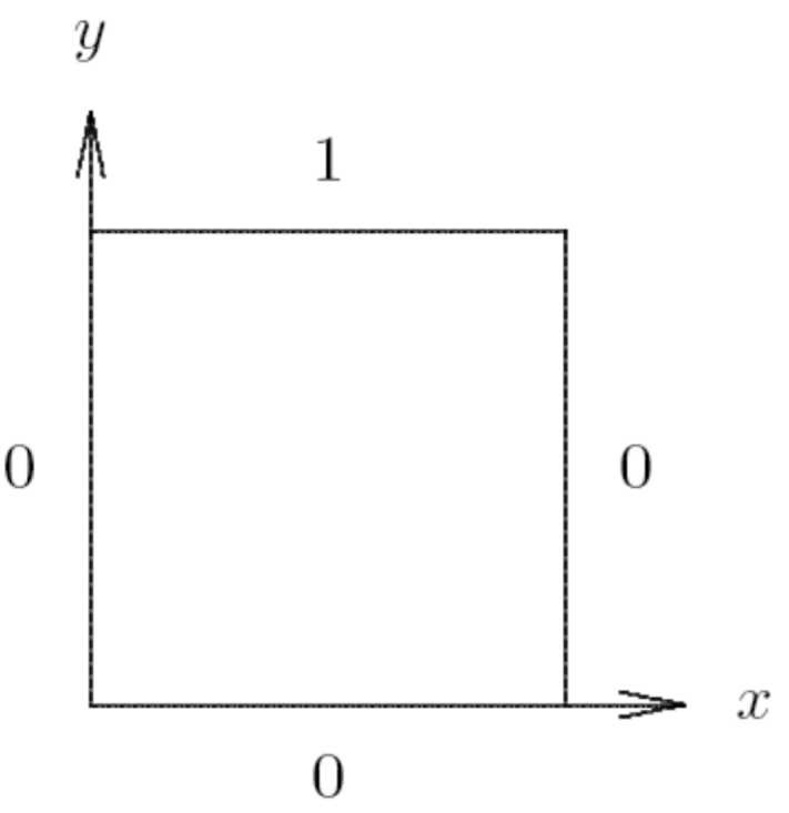
Consider the Laplace equation on the unit square:

$u_{xx} + u_{yy} = 0, \quad 0 \leq x \leq 1, \quad 0 \leq y \leq 1$

Page 40: Diagram showing the unit square with boundary conditions.

• Top boundary ($y = 1$): $u = 1$
• Left boundary ($x = 0$): $u = 0$
• Right boundary ($x = 1$): $u = 0$
• Bottom boundary ($y = 0$): $u = 0$

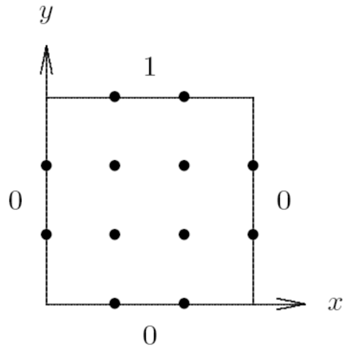
Mesh Definition

Page 41: Diagram showing the discrete mesh with interior and boundary points.

Interior grid points:
$(x_i, y_j) = (ih, jh), \quad i, j = 1, \ldots, n$

where $n = 2$ and $h = \frac{1}{n+1} = \frac{1}{3}$.

Finite Difference Approximation

Let $u_{i,j}$ be an approximation to the true solution $u(x_i, y_j)$.

Boundary values: $u_{i,j}$ where either $i$ or $j$ is $0$ or $n+1$.

Replace second derivatives with second-order centered differences:

$\frac{u_{i+1,j} - 2u_{i,j} + u_{i-1,j}}{h^2} + \frac{u_{i,j+1} - 2u_{i,j} + u_{i,j-1}}{h^2} = 0$

where $i, j = 1, \ldots, n$.

Simplifying:
$u_{i+1,j} - 2u_{i,j} + u_{i-1,j} + u_{i,j+1} - 2u_{i,j} + u_{i,j-1} = 0$
$\boxed{4u_{i,j} - u_{i-1,j} - u_{i+1,j} - u_{i,j-1} - u_{i,j+1} = 0}$

Analogy: This equation says that at equilibrium (steady state), the value at each interior point is the average of its four neighbors (up, down, left, right). Like a stretched rubber membrane - each point settles at the average height of its neighbors.

System of Equations

Writing out the four equations explicitly (for $n=2$, we have 4 interior points):

$4u_{1,1} - u_{0,1} - u_{2,1} - u_{1,0} - u_{1,2} = 0$
$4u_{2,1} - u_{1,1} - u_{3,1} - u_{2,0} - u_{2,2} = 0$
$4u_{1,2} - u_{0,2} - u_{2,2} - u_{1,1} - u_{1,3} = 0$
$4u_{2,2} - u_{1,2} - u_{3,2} - u_{2,1} - u_{2,3} = 0$

บางอันเรารู้ว่าเพราะเป็น Boundary

Matrix Form