"Dive into the origin of assembler language - This is how you control the computer"

Table of Contents

1. Turing Machines (TM)
2. Combining TMs
3. Recursive languages
4. Recursive Functions
5. Recursively Enumerable Languages
6. Extensions of Turing Machines

1. Turing Machines (TM)

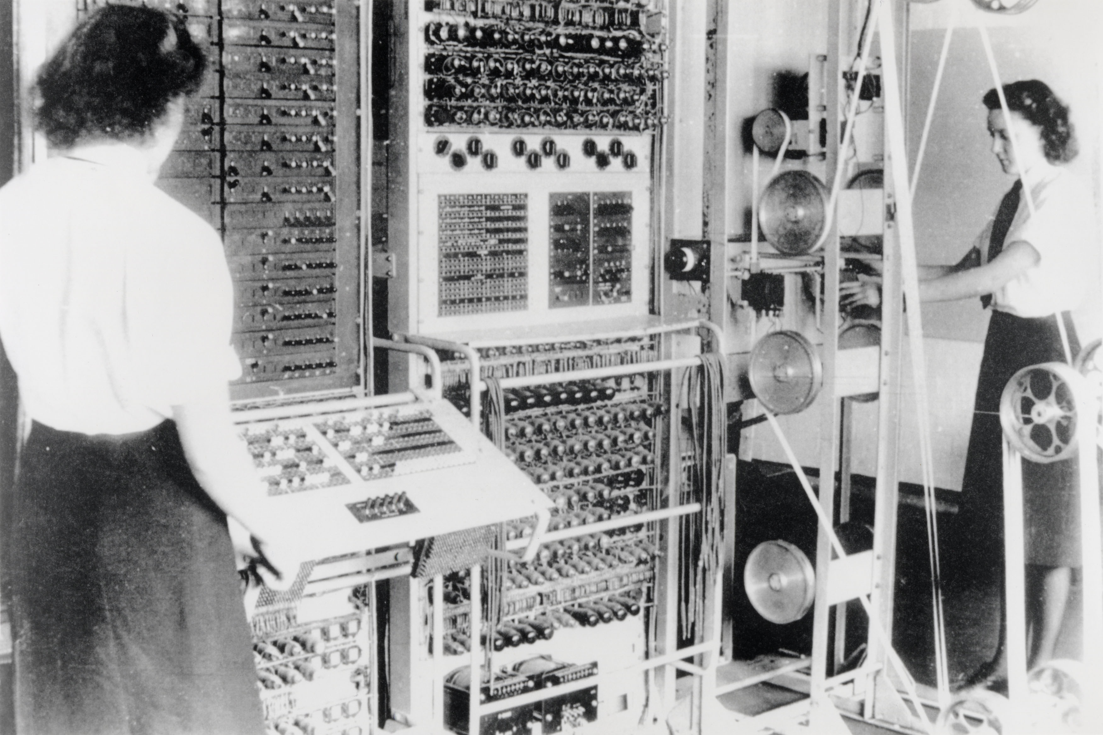
Historical Context: The Colossus Computer

Real-life Connection: The Colossus was one of the first electronic digital programmable computers. Built during WWII at Bletchley Park, it was used for codebreaking. The image in the lecture shows operators working with this massive machine that used vacuum tubes and had magnetic tape for memory storage.

Components of a Turing Machine

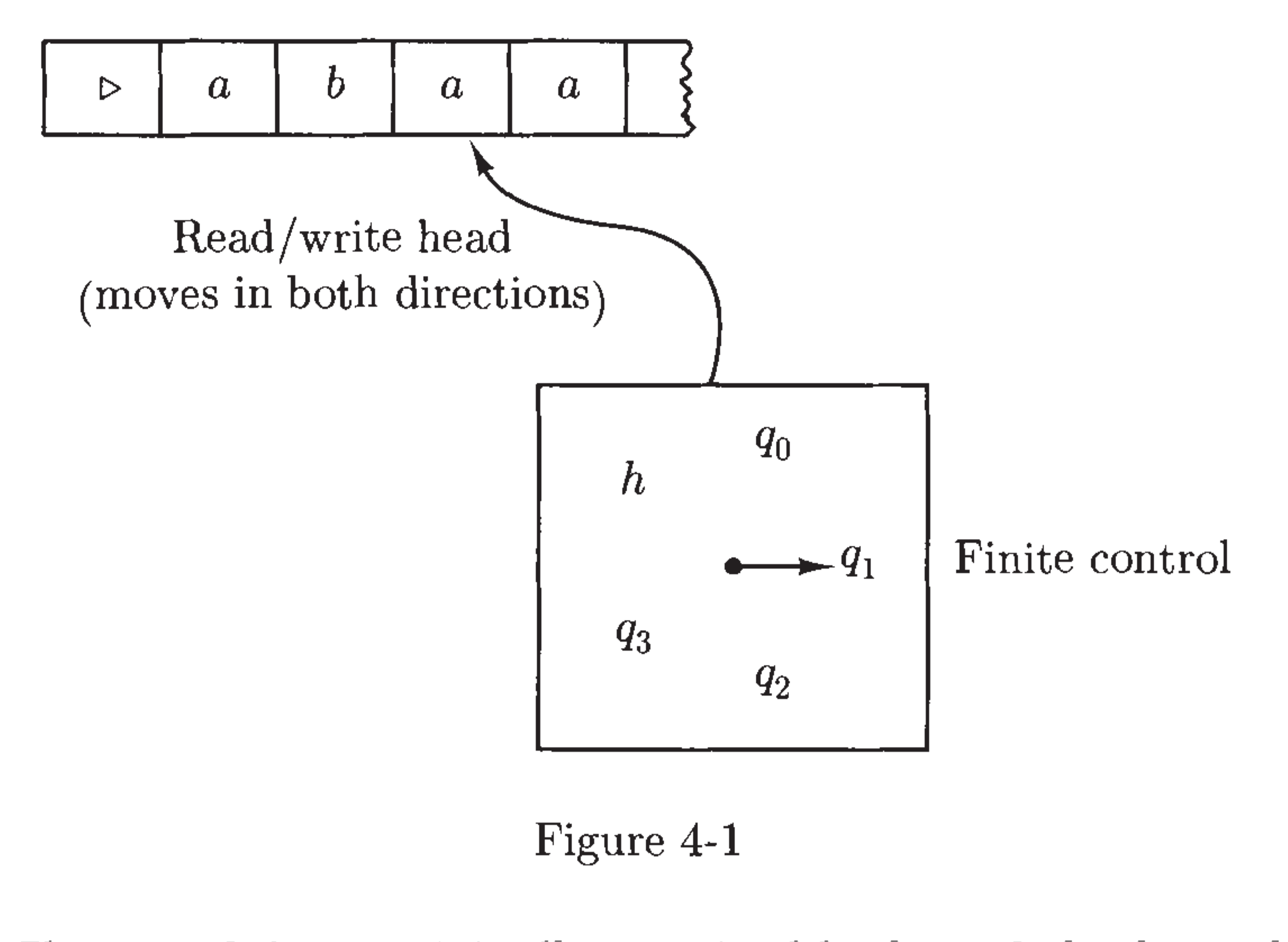
A Turing Machine consists of:

1. CPU (Finite Control)
   • State register that memorizes the current stage of the machine
   • Contains the program (instruction set) of the machine
   • Has states: $q_0, q_1, q_2, q_3, h$ (where $h$ is the halting state)
2. Memory (Tape)
   • But back then we didn't have RAM!
   • We have magnetic tape instead
   • Infinite tape divided into cells
   • Each cell can contain a symbol from the alphabet
3. Read/Write Head
   • Can move in both directions (left or right)
   • Can read the current symbol
   • Can write a new symbol

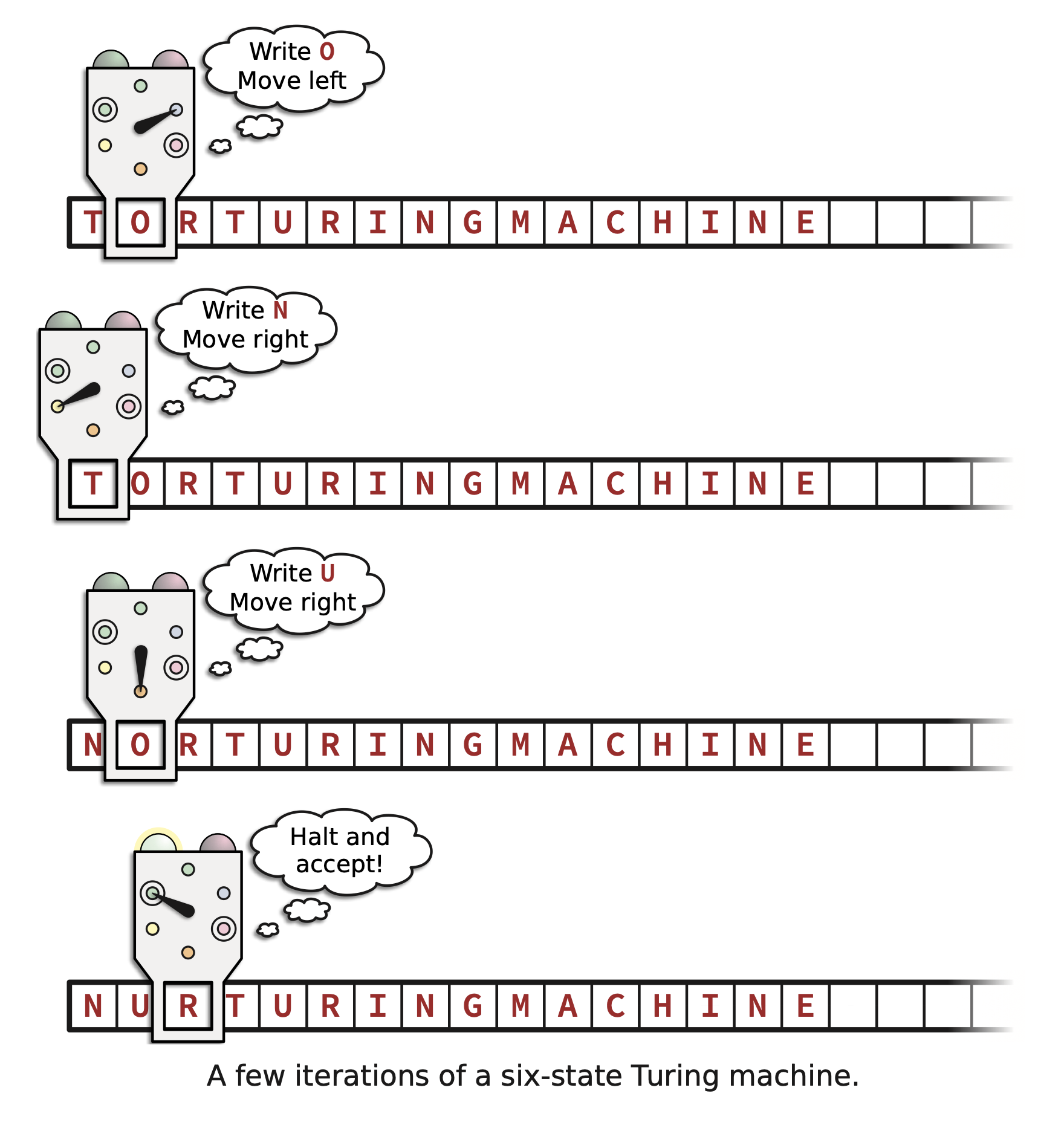
Analogy: Think of a Turing Machine like an old cassette tape player. The tape moves left and right, there's a read/write head that can detect and change what's on the tape, and there's a control unit that decides what to do based on what it reads.

Formal Definition

มาเริ่มกันละว่า How can we define those components mathematically

Definition: A Turing machine is a 5-tuple $\boxed{M = (K, \Sigma, \delta, s, H)}$ where:

• $K$ is a finite set of states
• $\Sigma$ is an alphabet containing:
  • The blank symbol $\sqcup$ (represents empty cells)
  • The left end symbol $\triangleright$ (marks the start of the tape)
  • But NOT containing the symbols $\rightarrow$ and $\leftarrow$ (these are for movement)
• $s \in K$ is the initial state (starting point)
• $H \subseteq K$ is the set of halting states (when machine stops)
  • It gets out of an infinite loop when it reaches a halting state
• $\delta$ is the transition function (the program/instruction set):
  $\boxed{\delta: (K - H) \times \Sigma \rightarrow K \times (\Sigma \cup \{\leftarrow, \rightarrow\})}$
  With these constraints:
  • For all $q \in K - H$, there exists $p$ such that $\delta(q, \triangleright) = (p, \rightarrow)$
    • Meaning: It never writes $\triangleright$ onto the memory. The tape start is always $\triangleright$, and when you see it, you can only move right.
    • Write down อะไรก็ได้ แต่จะ Write $\triangleright$ หรอ ตลก55555
  • For all $q \in K - H$ and $a \in \Sigma - \{\triangleright\}$, if $\delta(q, a) = (p, b)$ then $b \neq \triangleright$
    • Meaning: Only one tape start exists, and it's always on the left

Exam Tip: Remember the mnemonic:

• K = Kollection of states
• $\Sigma$ = Symbols (alphabet)
• $\delta$ = Decisions (transitions)
• s = start
• H = Halt

Understanding the Transition Function

The transition function $\delta$ takes:

• Input: (current state, input symbol)
• Output: (next state, action)

Where action can be:

• A symbol to write (replacing current cell content)
• $\leftarrow$: move pointer to the left (LHS)
• $\rightarrow$: move pointer to the right (RHS)

Important constraints:

• Start of tape marker ($\triangleright$) is never written by the machine (นี่แหละ ๆ)
• When seeing $\triangleright$, the head must move right

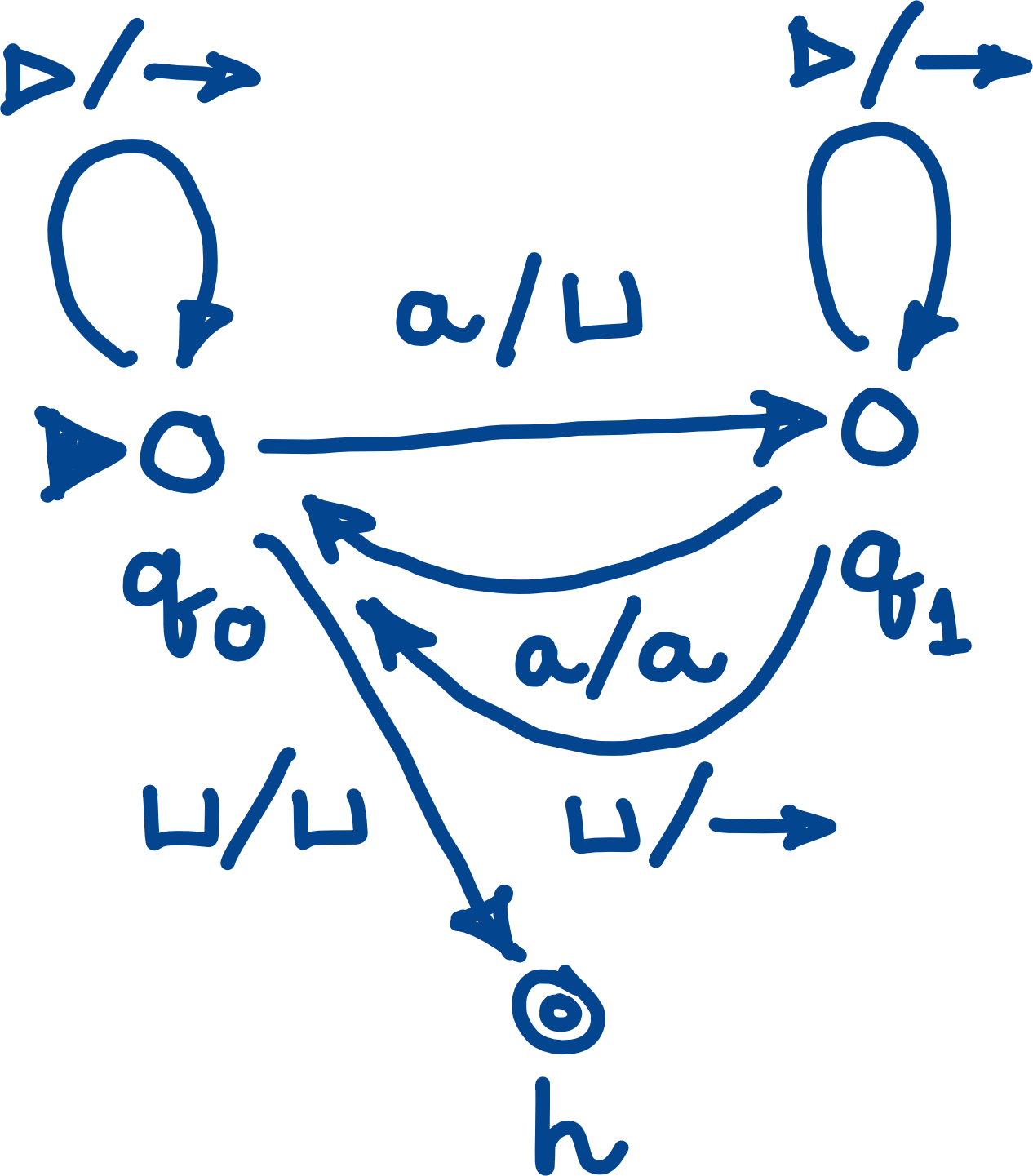
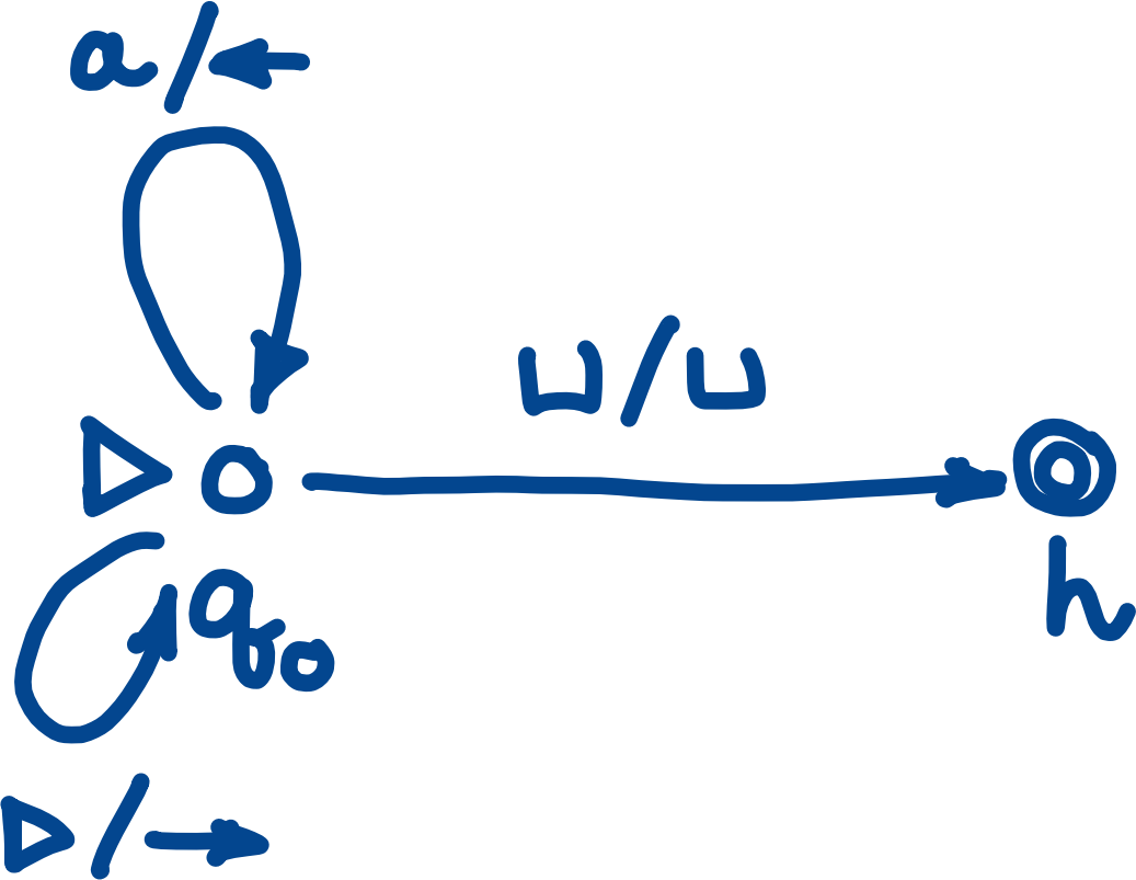
Example 4.1.1: Simple Turing Machine

Consider the Turing machine $M = (K, \Sigma, \delta, s, \{h\})$ where:

• $K = \{q_0, q_1, h\}$
• $\Sigma = \{a, \sqcup, \triangleright\}$
• $s = q_0$ (initial state)
• $h$ is the halting state

Transition Function $\delta$ (given by table):

Transition Diagram:

What this machine does:

• Starts at $q_0$
• Replaces every $a$ with blank ($\sqcup$)
• Effectively erases all $a$'s from the tape

Example Execution:

ใน Lecture PDF มันไม่มี Blank หลัง start แต่คุ้น ๆ หลัง ๆ อาจารย์บอกให้มี

Starting configuration: $(q_0, \triangleright \sqcup aaaa)$

Insight: This is essentially a "clear all a's" program - like find and replace in a text editor, but at the machine level!

Example 4.1.2: Even Simpler Machine

Consider $M = (K, \Sigma, \delta, s, H)$ where:

• $K = \{q_0, h\}$
• $\Sigma = \{a, \sqcup, \triangleright\}$
• $s = q_0$
• $H = \{h\}$

Transition Table:

Transition Diagram:

What this machine does:

• Moves left when seeing $a$
• Halts when seeing blank
• This machine scans left until it finds a blank

Example 4.1.3: Recognizing Even-Length Strings

A Turing machine for accepting $L = \{\omega \in \{a,b\}^* \mid |\omega| \text{ is even}\}$

• $K = \{s, q_0, q_1, y, n\}$ where $H = \{y, n\}$
  • $y$ = accept state
  • $n$ = reject state
• $\Sigma = \{a, b, \sqcup, \triangleright\}$
• Transition function $\delta$:

Transition Diagram:

         a,b→
        ┌────┐
        ↓    │
  ▷─○──→○────○
    s   q₀   q₁
   ⊔/→  │    │
        ↓⊔/⊔ ↓⊔/⊔
        ◎y   ◎n

Accepting computation for $aa$:

Initial config: (s, ▷⊔aa) ≠ (s, ▷⊔⊔ω)
                              ↑
                           cursor on input string

(s, ▷⊔aa) ⊢ₘ (q₀, ⊔aa) ⊢ₘ 
(q₁, ⊔aa) ⊢ₘ (q₀, ⊔aa⊔) ⊢ₘ 
(y, ⊔aa⊔)  STOP/HALT

Rejecting computation for $a$:

(s, ▷⊔a) ⊢ₘ (q₀, ⊔a) ⊢ₘ
(q₁, ⊔a⊔) ⊢ₘ (n, ⊔a⊔)  STOP/HALT

Exam Strategy: For simple state machine problems, always alternate between two states to count parity (even/odd). State $q_0$ = even, state $q_1$ = odd.

Real-life Connection: This is essentially TM ≡ Modern Computer. The Turing Machine is a theoretical model that captures what computers can do!

Configurations

Definition: Configuration

มันก็คือการเขียน การอ่าน ของ Turing machine นั่นแหละมั้ง

A configuration of a Turing machine $M = (K, \Sigma, \delta, s, H)$ is a member of:

$\boxed{K \times \triangleright \Sigma^* \times (\Sigma^* (\Sigma - \{\sqcup\}) \cup \{e\})}$

Breaking this down:

• Current state: $q \in K$
• Before the header: $\triangleright \omega_1$ (everything to the left including start marker)
• After the header: $\omega_2$ (everything to the right)
  • If it consists of only $\sqcup$'s or empty string, we can ignore it

Notation: Configuration is written as $(q, \omega_1 \underline{a} \omega_2)$ where:

• $q$ = current state
• $\triangleright \omega_1$ = tape content before head
• $\underline{a}$ = symbol under the head (current cell)
• $\omega_2$ = tape content after head

Syntactic Sugar:

• $(q_1, \triangleright \sqcup abac\sqcup) = (q_1, \triangleright \sqcup a\underline{b}ac)$ (CHECK)
• The underline shows where the head is positioned

Computation Steps (Yields Relation)

Definition: Let $(q_1, \omega_1 a_1 u_1)$ and $(q_2, \omega_2 a_2 u_2)$ be configurations of $M$. Then:
$\boxed{(q_1, \omega_1 a_1 u_1) \vdash_M (q_2, \omega_2 a_2 u_2)}$
if and only if for some $b \in \Sigma \cup \{\leftarrow, \rightarrow\}$, $\delta(q_1, a_1) = (q_2, b)$ and one of the following cases holds:

Case 1: Write a symbol ($b \in \Sigma$)

• $b \in \Sigma, \omega_1 = \omega_2, u_1 = u_2$ and $a_2 = b$
• Meaning: Replace the cell's content with symbol $b$, stay in place

Example:
$(q_2, \triangleright \sqcup a\underline{b}ac\sqcup) \vdash_M (q_2, \triangleright \sqcup a\underline{\sqcup}ac\sqcup) \quad \text{if } \delta(q_2, b) = (q_2, \sqcup)$

Case 2a: Move left ($b = \leftarrow$, normal case)

• $b = \leftarrow, \omega_1 = \omega_2 a_2$, and either:
  • $u_2 = a_1 u_1$, if $a_1 \neq \sqcup$ or $u_1 \neq e$, or
  • $u_2 = e$, if $a_1 = \sqcup$ and $u_1 = e$

Example:

Case 2b: Move left (edge case with blanks)

• $u_2 = e$, if $a_1 = \sqcup$ and $u_1 = e$
• Empty strings - we can ignore them

Example:

Case 3a: Move right ($b = \rightarrow$, normal case)

• $b = \rightarrow, \omega_2 = \omega_1 a_1$, and either:
  • $u_1 = a_2 u_2$

Example:

Case 3b: Move right (edge case)

• $u_1 = u_2 = e$ and $a_2 = \sqcup$

Intuition: Think of configurations as "snapshots" of the machine at any point in time. The $\vdash_M$ symbol means "yields" or "steps to" - it shows how one snapshot transitions to the next.

Halted Configuration and Computation

แล้วหยุด กูจะหยุดมึงเอง!

Definition: Halted Configuration

A halted configuration is of the form:
$\boxed{(h, \omega_1 \underline{a} \omega_2) \text{ with } h \in H}$

• The machine returns a result when it reaches a halted configuration
• Result is whatever is on the tape at that moment

Definition: Computation

A computation is a sequence of configurations $C_1, C_2, \ldots, C_n$ such that:
$C_1 \vdash_M C_2 \vdash_M \cdots \vdash_M C_n$
We say that:

• The computation has length $n$
• $C_1$ yields $C_n$

Definition: Halting

$M$ is said to halt on input $\omega$ iff $(s, \triangleright \sqcup \omega)$ yields some halted configuration.
$\boxed{(s, \triangleright \sqcup \omega) \vdash_M^* (h, \triangleright \omega')}$
Where:

• $(s, \triangleright \sqcup \omega)$ = initial configuration
• $(h, \triangleright \omega')$ = final configuration (may not need to be the same)
• $\omega'$ = the result
• $\vdash_M^*$ means "yields in zero or more steps"

Important Note: The mem ctn (memory content) needs not be the same before and after computation.

Exam Tip: When tracing a computation:

1. Start with initial config: $(s, \triangleright \sqcup \omega)$
2. Apply transitions step by step
3. Stop when you reach a halting state
4. Check if the final configuration is what you expect

2. Combining TMs

Symbol Writing Machines

• For each symbol $a \in \Sigma \cup \{\leftarrow, \rightarrow\} - \{\triangleright\}$, $M_a$ is a Turing machine which writes the symbol $a$ into the scanned tape square.
• Formal definition: $M_a = (\{s, h\}, \Sigma, \delta, s, \{h\})$ where $\delta(s, b) = (h, a)$ for each $b \in \Sigma - \{\triangleright\}$.

Mnemonics (Short Notations)

To keep things simple, we write:

• $a$ for $M_a$ → write '$a$' to the current cell
• $L$ for $M_\leftarrow$ → move pointer to LHS (Left)
• $R$ for $M_\rightarrow$ → move pointer to RHS (Right)

Special composite machines:

• $L_\sqcup$: Finds the first blank square to the left of the currently scanned symbol

- Scan left until blank found

• $R_\sqcup$: Finds the first blank square to the right of the currently scanned symbol

- Scan right until blank found

Atomic vs Composite Machines

• If you have two Turing machines, you can connect them together!

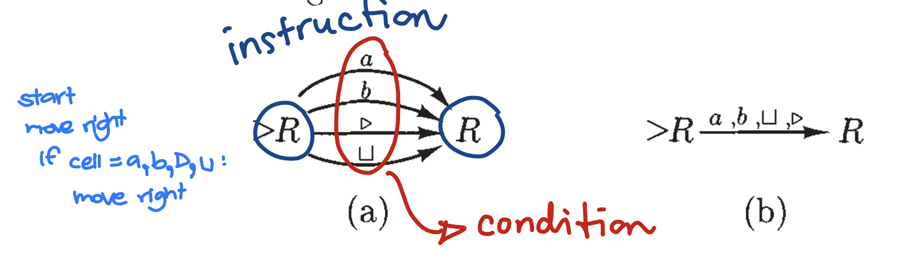
Example 4.1.5: Sequential Composition

Machine: $RR$ or $R^2$

Diagram:

What it does:

1. Start: move right
2. If cell is $a$, $b$, $\sqcup$, or $\triangleright$: move right again

Shorthand notation:

• Unlabeled arrow = works for all symbols in alphabet
• Can omit arrow entirely by juxtaposing: $R \rightarrow R$ becomes just $RR$

Note: "Program" states are hidden - each node is a sequence of commands, each edge is a peek to the current cell.

Example trace:

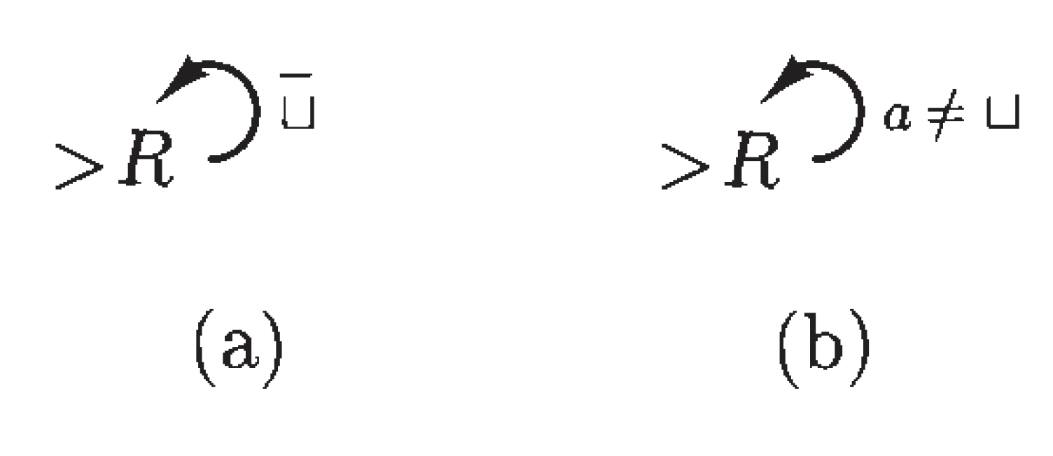
Example 4.1.6: Conditional Movement ($R_\sqcup$)

Machine: $R_\sqcup$ - moves right until blank found

Diagram:

Alternative notation:

Where $a \neq \sqcup$ is read as "any symbol $a$ other than $\sqcup$"

What it does:

• Scan right
• If current cell is NOT blank: keep moving right
• If current cell IS blank: halt

Advantage of $a \neq \sqcup$ notation: The variable $a$ can be used elsewhere in the diagram

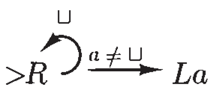
Example 4.1.6 continuation: Copy and Move

• ตรง $R_\sqcup$ มี Self-loop ถ้าเป็น $\sqcup$
  What this does:

1. Scan right until blank found ($R_\sqcup$)
2. If found a non-blank symbol $a$ (store it as variable)
3. Move left ($L$)
4. Write that symbol $a$ at the new position

Example 4.1.7: Find Marked or Unmarked Squares

Four useful machines for finding specific squares:

(a) $R_\sqcup$: Find first blank square to the right

         ⊔
     ┌────────┐
     ↓        │
  ▷→ R

(b) $L_\sqcup$: Find first blank square to the left

         ⊔
     ┌────────┐
     ↓        │
  ←─ L

(c) $R_{\overline{\sqcup}}$: Find first non-blank square to the right

         ⊔
     ┌────────┐
     ↓        │
  ▷→ R

(d) $L_{\overline{\sqcup}}$: Find first non-blank square to the left

         ⊔
     ┌────────┐
     ↓        │
  ←─ L

Summary Table:

Example 4.1.8: The Copying Machine ($C$) (CHECK!)

Purpose: Copy input string - transforms $\sqcup \omega \underline{\sqcup}$ into $\sqcup \omega \sqcup \omega \underline{\sqcup}$

Starting condition:

• Input: String $\omega$ containing only non-blank symbols (possibly empty)
• Tape: $\omega$ on an otherwise blank tape with one blank square to its left
• Head: Positioned on the blank square to the left of $\omega$

Result: Eventually stops with $\omega \sqcup \omega$ on an otherwise blank tape

Diagram:

\usepackage{tikz, amsmath, amssymb}
\usetikzlibrary{arrows.meta, positioning}
 
\begin{document}
 
\begin{tikzpicture}[node distance=3cm, >=Stealth, thick]
 
% Define nodes
\node (Lblank) {$>L_{\sqcup}$};
\node (R) [right=of Lblank] {$R$};
\node (Rblank) [below=of R] {$R_{\sqcup}$};
\node (copy) [right=4cm of R] {$\sqcup R_{\sqcup}^2 a L_{\sqcup}^2 a$};
 
% Arrows
\draw[->] (Lblank) -- (R);
\draw[->] (R) -- node[above] {$a \neq \sqcup$} (copy);
\draw[->] (R) -- node[left] {$\sqcup$} (Rblank);
 
% Up-straight-down loop (Π-shape)
\draw[->] (copy.north) |- ++(0,1.8) -| (R.north);
 
\end{tikzpicture}
 
\end{document}

Full Trace

How it works (Copy works backwards):

Starting tape: $\triangleright \sqcup abc$

1. $L_\sqcup$: Move left to find first blank
   • $\triangleright \sqcup abc$ → head at first blank
2. Read symbol (if $a \neq \sqcup$): Store current symbol
   • Found symbol $c$, store it as variable $a$
3. Replace with blank: Write $\sqcup$ to mark as "copied"
   • $\triangleright \sqcup ab\sqcup$
4. $R_\sqcup$: Move right until blank found
   • $\triangleright \sqcup ab\sqcup$ → head at rightmost blank
5. Write symbol $a$: Write the stored symbol
   • $\triangleright \sqcup ab\sqcup c$
6. $L_\sqcup$: Move left to find blank (the marker)
   • Back to the marked position
7. Check if done: If current symbol is $\sqcup$, we're at start → halt
   • Otherwise, continue from step 2 with next symbol

Complete trace for input $abc$: (Check ด้วย ทำไมมัน clear หมด)
ถ้าว่างก็ทำหน่อยว้อย

Final result: ▷⊔abc⊔cba (reversed copy)

Insight: This machine copies string but in reverse order! It's like "lives program" - cursor enter me exit.

Example 4.1.9: The Right-Shifting Machine ($S_\rightarrow$) (CHECK)

Purpose: Transforms $\sqcup \omega \underline{\sqcup}$ into $\sqcup \sqcup \omega \underline{\sqcup}$ (shifts string one position right)

Diagram:

         a≠⊔
     ┌────────┐
     ↓        │
  ▷→ L  ────⊔──→ ⊔ → R_⊔ → a → L_{\overline{⊔}}
     ↑                              │
     └──────────────────────────────┘

How it works:

Starting tape: ▷⊔abc

1. Move to rightmost symbol
2. Remember it (call it $a$)
3. Replace with blank (shift it right)
4. Move left to previous non-blank
5. Remember that symbol
6. Write the previous symbol ($a$) there
7. Repeat until all shifted

Example trace:

▷⊔abc  ⊢ [to end]      ▷⊔abc   
       ⊢ [a=c]         ▷⊔ab⊔   (store c, shift)
       ⊢ [R_⊔, write]  ▷⊔ab⊔c  (write at next blank)
       ⊢ [back]        ▷⊔ab⊔c
       ⊢ [a=b]         ▷⊔a⊔⊔c  (store b, shift)
       ⊢ [write]       ▷⊔a⊔bc  
       ⊢ [a=a]         ▷⊔⊔⊔bc  (store a, shift)
       ⊢ [write]       ▷⊔⊔abc  (DONE!)

Result: ▷⊔⊔abc (shifted right by one position)

Analogy: Like pushing text to the right by inserting a space at the beginning.

Example 4.1.10: Erasing Machine (CHECK)

Purpose: Erase all $a$'s from the tape (from Example 4.1.1)

Simple diagram:

\usepackage{tikz, amsmath, amssymb}
\usetikzlibrary{arrows.meta, positioning}
 
\begin{document}
 
\begin{tikzpicture}[node distance=2cm, >=Stealth, thick]
 
% Nodes
\node (Rstart) {$>R$};
\node (blank) [right=of Rstart] {$\sqcup$};
 
% Main arrow (R -> blank)
\draw[->] (Rstart) -- node[below] {$a$} (blank);
 
% Sharp up–across–down arrow (blank -> R)
\draw[->] (blank.north) |- ++(0,1) -| (Rstart.north);
 
\end{tikzpicture}
 
\end{document}

What it does:

1. If current cell is $a$: replace with blank, stay in state
2. If current cell is blank: halt
3. Otherwise: move right

This is the "clear the tape" operation - removes all occurrences of symbol $a$.

Rules for Combining Machines (Formal Definition)

Suppose we have three Turing machines:

• $M_1 = (K_1, \Sigma, \delta_1, s_1, H_1)$
• $M_2 = (K_2, \Sigma, \delta_2, s_2, H_2)$
• $M_3 = (K_3, \Sigma, \delta_3, s_3, H_3)$

Combined Machine Structure

  ▷ M₁ ──a──→ M₂
       │
       b
       ↓
      M₃

How it works:

1. Let $M_1$ work until it halts
2. Peek the current cell
3. If the cell contains $a$, let $M_2$ work
4. If the cell contains $b$, let $M_3$ work

Formal Construction

The combined machine $M = (K, \Sigma, \delta, s, H)$ where:

• $K = K_1 \cup K_2 \cup K_3$ (union of all states)
• $s = s_1$ (start with first machine's start state)
• $H = H_2 \cup H_3$ (halt when any component halts)

For each $\sigma \in \Sigma$, $q \in K - H$, $\delta(q, \sigma)$ is defined as follows:

1. If $q \in K_1 - H_1$ (non-halting state of $M_1$):
   • $\delta(q, \sigma) = \delta_1(q, \sigma)$
   • Use $M_1$'s transitions
2. If $q \in K_2 - H_2$ (non-halting state of $M_2$):
   • $\delta(q, \sigma) = \delta_2(q, \sigma)$
   • Use $M_2$'s transitions
3. If $q \in K_3 - H_3$ (non-halting state of $M_3$):
   • $\delta(q, \sigma) = \delta_3(q, \sigma)$
   • Use $M_3$'s transitions
4. If $q \in H_1$ (halting state of $M_1$):
   • $\delta(q, \sigma) = (s_2, \sigma)$ if $\sigma = a$ (jump to $M_2$)
   • $\delta(q, \sigma) = (s_3, \sigma)$ if $\sigma = b$ (jump to $M_3$)
   • $\delta(q, \sigma) \in H$ otherwise (halt if no condition matches)

Programming Analogy: This is like an if-clause in programming:

def combined_machine(tape):
    M1.run(tape)  # Run M1 until it halts
    symbol = tape.read_current()
    if symbol == 'a':
        M2.run(tape)  # JMP to M2
    elif symbol == 'b':
        M3.run(tape)  # JMP to M3
    else:
        halt()  # Stop if no condition matches

Assembly Language Equivalent:

• JMP (unconditional jump)
• JZ (jump if zero)
• JNZ (jump if not zero)
• These are the "branching" or "flowchart" operations

Quick Reference: Composite Machine Notations

Diagram notation:

• Initial Configuration: $\triangleright \sqcup \omega$
• Condition/Branch: Decision points (if-then)
• Self-loop: Repeating state

3. Recursive Languages

3.1 Definition: Accepting and Rejecting Configurations

Context: Recursive languages can be defined as a recursive function (recursive algorithm)

Addition as recursion example:
f(a,b) = f(a+1, b-1) \text{ if } b > 0$$$$f(a,0) = a

Definition: Given is a Turing machine $M = (K, \Sigma, \delta, s, H)$ with $\boxed{H = \{y, n\}}$.

• Any halting configuration whose state is $\color{green}y$ is said to be an accepting configuration $(y, \_)$
• A halting configuration whose state is $\color{red}n$ is said to be a rejecting configuration $(n, \_)$

An initial configuration is of the form $(s, \triangleright \sqcup \omega)$

For an input $\omega \in (\Sigma - \{\sqcup, \triangleright\})^*$, we say that:

• $M$ accepts $\omega$ if $(s, \triangleright \sqcup \omega)$ yields an accepting configuration
  $\vdash_M^* (y, \_)$
• $M$ rejects $\omega$ if $(s, \triangleright \sqcup \omega)$ yields a rejecting configuration
  $\vdash_M^* (n, \_)$

Important Note:

• ถ้าจาก Initial config ถ้าไปถึง $y,n$ ได้ก็คือ Accepted
• แต่ถ้าไม่ถึงทั้งคู่ $y,n$ เช่นอาจจะติด Loop ก็คือจะไม่ได้คำตอบ
• If $M$ gets stuck in an $\infty$-loop, we won't get answer

Definition: Deciding a Language (Recursive Languages)

Definition: Let $\Sigma_0 \subseteq \Sigma - \{\sqcup, \triangleright\}$ be an alphabet, called input alphabet. We say that $M$ decides a language $L \subseteq \Sigma_0^*$ if for any string $\omega \in \Sigma_0^*$:

\begin{align*}
&\triangleright R \xrightarrow{a} dR \xrightarrow{b} dL_\sqcup \
&\text{where:} \
&\quad R: \text{Move right (self-loop on } d\text{)} \
&\quad dR: \text{Replace } a \text{ with } d\text{, then move right (self-loop on } a,d\text{)} \
&\quad dL_\sqcup: \text{Replace } b \text{ with } d\text{, then scan left to blank}
\end{align*}

\begin{align*}
&\checkmark \triangleright \sqcup \underline{a}abb \vdash_R && \text{[start, move to first symbol]} \
&\checkmark \triangleright \sqcup \underline{d}abb \vdash_d && \text{[replace } a \text{ with } d\text{]} \
&\checkmark \triangleright \sqcup d\underline{a}bb \vdash_R && \text{[move right]} \
&\checkmark \triangleright \sqcup da\underline{b}b \vdash_R && \text{[skip over remaining } a\text{]} \
&\checkmark \triangleright \sqcup da\underline{d}b \vdash_d && \text{[replace first } b \text{ with } d\text{]} \
&\checkmark \triangleright \sqcup \underline{d}adb \vdash_{L_\sqcup} && \text{[return to left blank]} \
&\checkmark \triangleright \sqcup d\underline{a}db \vdash_R && \text{[move right, find next } a\text{]} \
&\checkmark \triangleright \sqcup d\underline{d}db \vdash_R && \text{[skip } d\text{]} \
&\checkmark \triangleright \sqcup dd\underline{d}b \vdash_R && \text{[skip } d\text{]} \
&\checkmark \triangleright \sqcup ddd\underline{b} \vdash_R && \text{[find } b\text{]} \
&\checkmark \triangleright \sqcup ddd\underline{d} \vdash_d && \text{[replace } b \text{ with } d\text{]} \
&\checkmark \triangleright \underline{\sqcup}dddd \vdash_{L_\sqcup} && \text{[return to left]} \
&\checkmark \triangleright \sqcup \underline{d}ddd \vdash_R && \text{[try to find } a\text{]} \
&\checkmark \triangleright \sqcup dddd\underline{\sqcup} \vdash_{R_\sqcup}^* && \text{[all } d\text{, no more } a\text{]} \
&\checkmark \triangleright \sqcup dddd\underline{\sqcup} \vdash_y && \text{[ACCEPT!]} \
&\triangleright \sqcup dddd\sqcup
\end{align*}

\begin{align*}
&\text{From Figure 4-11:} \
&\triangleright R \xrightarrow{a} dR \xrightarrow{b} dR \xrightarrow{c} dL_\sqcup \
&\text{Self-loops: } d \text{ on each state}
\end{align*}

\begin{align*}
\triangleright \sqcup \underline{a}abbcc &\vdash_R \triangleright \sqcup \underline{d}abbcc && [R: \text{find } a] \
\triangleright \sqcup d\underline{a}bbcc &\vdash_R \triangleright \sqcup da\underline{b}bcc && [dR: \text{skip } a] \
\triangleright \sqcup da\underline{d}bcc &\vdash_d \triangleright \sqcup dad\underline{b}cc && [dR: \text{find } b] \
\triangleright \sqcup dadb\underline{c}c &\vdash_R \triangleright \sqcup dadb\underline{d}c && [dR: \text{find } c] \
\triangleright \underline{\sqcup}dadbd &\vdash_{L_\sqcup} && [dL_\sqcup: \text{back to start}] \
\triangleright \sqcup \underline{d}adbdc &\vdash_R && [R: \text{skip } d] \
\triangleright \sqcup d\underline{a}dbdc &\vdash_R && [R: \text{find next } a] \
\triangleright \sqcup d\underline{d}dbdc &\vdash_d && [\text{replace } a \text{ with } d] \
\triangleright \sqcup dd\underline{d}bdc &\vdash_R && [dR: \text{skip } d] \
\triangleright \sqcup ddd\underline{b}dc &\vdash_R && [dR: \text{find } b] \
\triangleright \sqcup ddd\underline{d}dc &\vdash_d && [\text{replace } b \text{ with } d] \
\triangleright \sqcup dddd\underline{d}c &\vdash_R && [dR: \text{skip } d] \
\triangleright \sqcup ddddd\underline{c} &\vdash_R && [dR: \text{find } c] \
\triangleright \sqcup ddddd\underline{d} &\vdash_d && [\text{replace } c \text{ with } d] \
\triangleright \underline{\sqcup}dddddd &\vdash_{L_\sqcup} && [dL_\sqcup: \text{back to start}] \
\triangleright \sqcup \underline{d}ddddd &\vdash_R && [R: \text{try find } a] \
\triangleright \sqcup dddddd\underline{\sqcup} &\vdash_{R_\sqcup}^* && [\text{all } d\text{, no } a \text{ left}] \
\triangleright \sqcup dddddd\underline{\sqcup} &\vdash_y && \text{YES - ACCEPT}
\end{align*}

\begin{align*}
&R^z \xrightarrow{a} zR \xrightarrow{b} zR \xrightarrow{c} zR \xrightarrow{d} dL_\sqcup \
&\text{With self-loops on: } a,z; \quad b,z; \quad c,z
\end{align*}

\begin{align*}
&\text{DFA: } p \xrightarrow{a} q \
&\text{TM: } \delta'(p,a) = (\delta(p,a), \rightarrow) = (q, \rightarrow)
\end{align*}

\begin{align*}
&\triangleright R_\sqcup \begin{cases}
0 \rightarrow 1 \
1 \rightarrow 0
\end{cases} \text{ (go to last digit)} \
&\text{then: } \begin{cases}
0 \rightarrow 1 \text{ and halt} \
1 \rightarrow 0 \text{ and } L \text{ (carry)} \
\sqcup \rightarrow 1S_\rightarrow L_\sqcup \text{ (overflow: add digit)}
\end{cases}
\end{align*}

\begin{align*}
\triangleright \underline{\sqcup}100 &\vdash_{R_\sqcup} \triangleright \sqcup 100\underline{\sqcup} && [\text{move to last digit}] \
\triangleright \sqcup 100\underline{\sqcup} &\vdash_L \triangleright \sqcup 10\underline{0} && [\text{last digit is } 0] \
\triangleright \sqcup 10\underline{1} &\vdash && [\text{change } 0 \text{ to } 1, \text{ halt}]
\end{align*}

\begin{align*}
\triangleright \underline{\sqcup}101 &\vdash_{R_\sqcup} \triangleright \sqcup 101\underline{\sqcup} && [\text{go to end}] \
\triangleright \sqcup 101\underline{\sqcup} &\vdash_L \triangleright \sqcup 10\underline{1} && [\text{last digit}] \
\triangleright \sqcup 10\underline{0} &\vdash_L \triangleright \sqcup 1\underline{0}0 && [\text{change } 1 \text{ to } 0\text{, carry left}] \
\triangleright \sqcup 1\underline{1}0 &\vdash && [\text{change } 0 \text{ to } 1\text{, halt}]
\end{align*}

\begin{align*}
\triangleright \underline{\sqcup}111 &\vdash_{R_\sqcup} \triangleright \sqcup 111\underline{\sqcup} \
\triangleright \sqcup 111\underline{\sqcup} &\vdash_L \triangleright \sqcup 11\underline{1} && [\text{last digit is } 1] \
\triangleright \sqcup 11\underline{0} &\vdash_L \triangleright \sqcup 1\underline{1}0 && [\text{change to } 0\text{, carry}] \
\triangleright \sqcup 1\underline{0}0 &\vdash_L \triangleright \sqcup \underline{1}00 && [\text{change to } 0\text{, carry}] \
\triangleright \sqcup \underline{0}00 &\vdash_L \triangleright \underline{\sqcup}000 && [\text{change to } 0\text{, carry}] \
\triangleright \underline{\sqcup}1000 &\vdash_{1S_\rightarrow} && [\text{overflow: prepend } 1] \
\triangleright \sqcup \underline{1}000 &\vdash_{L_\sqcup} && [\text{shift right and add } 1]
\end{align*}

\begin{align*}
&\text{Regular} \subset \text{Context-Free} \subset \text{Recursive} \subset \text{Recursively Enumerable} \
&\text{(FSA)} \qquad \text{(PDA)} \qquad\qquad \text{(TM always halts)} \quad \text{(TM may not halt)}
\end{align*}