3.1 Searching for Solutions

Problem-solving agents find solutions by conducting search using the following algorithm:

Basic Search Algorithm Steps

1. Initialize
   
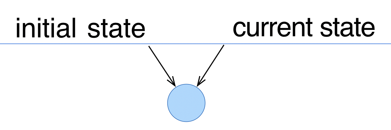
   • Start from the initial state
   • Set it as the current state
2. Expand
   
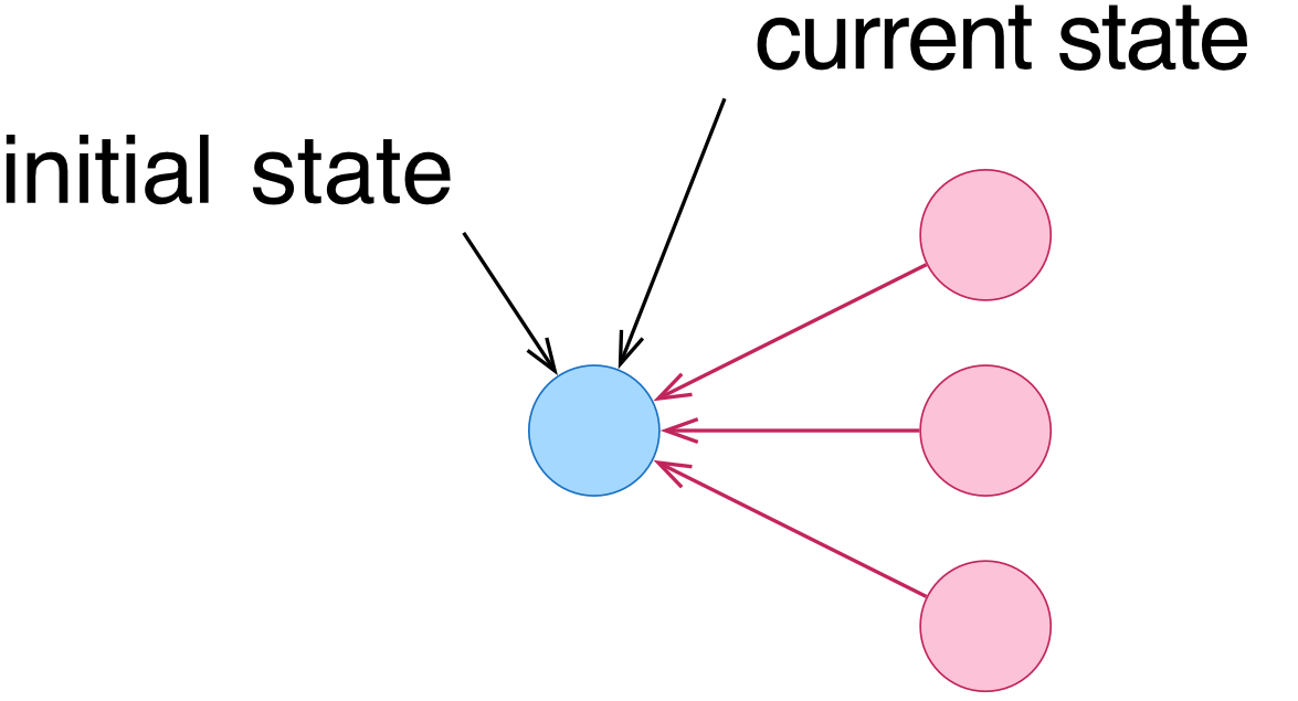
   • Apply all possible actions to the current state
   • Generate the set of successors
   • Keep them in a data structure called frontier
3. Select
   
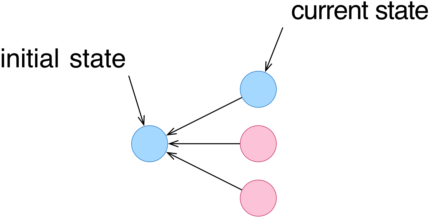
   • Choose one successor from the frontier
   • Set it as the new current state
4. Iterate
   
   
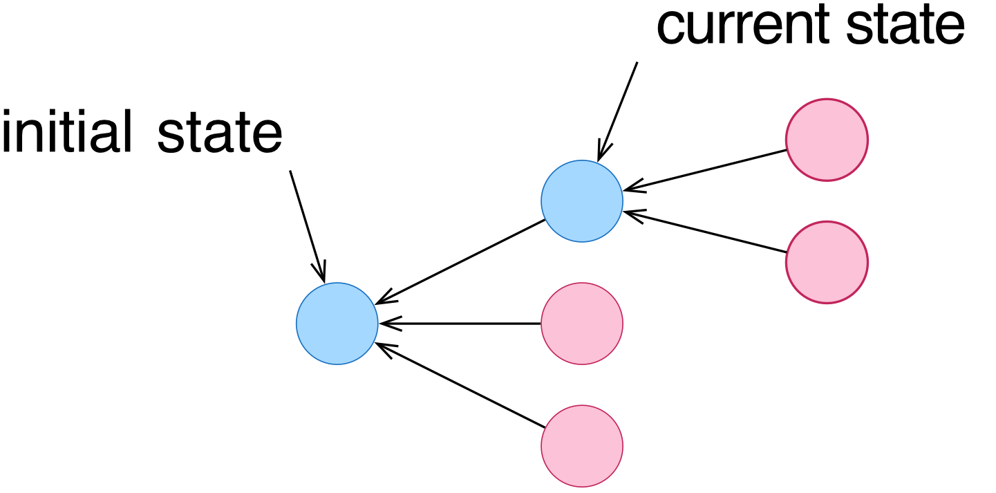
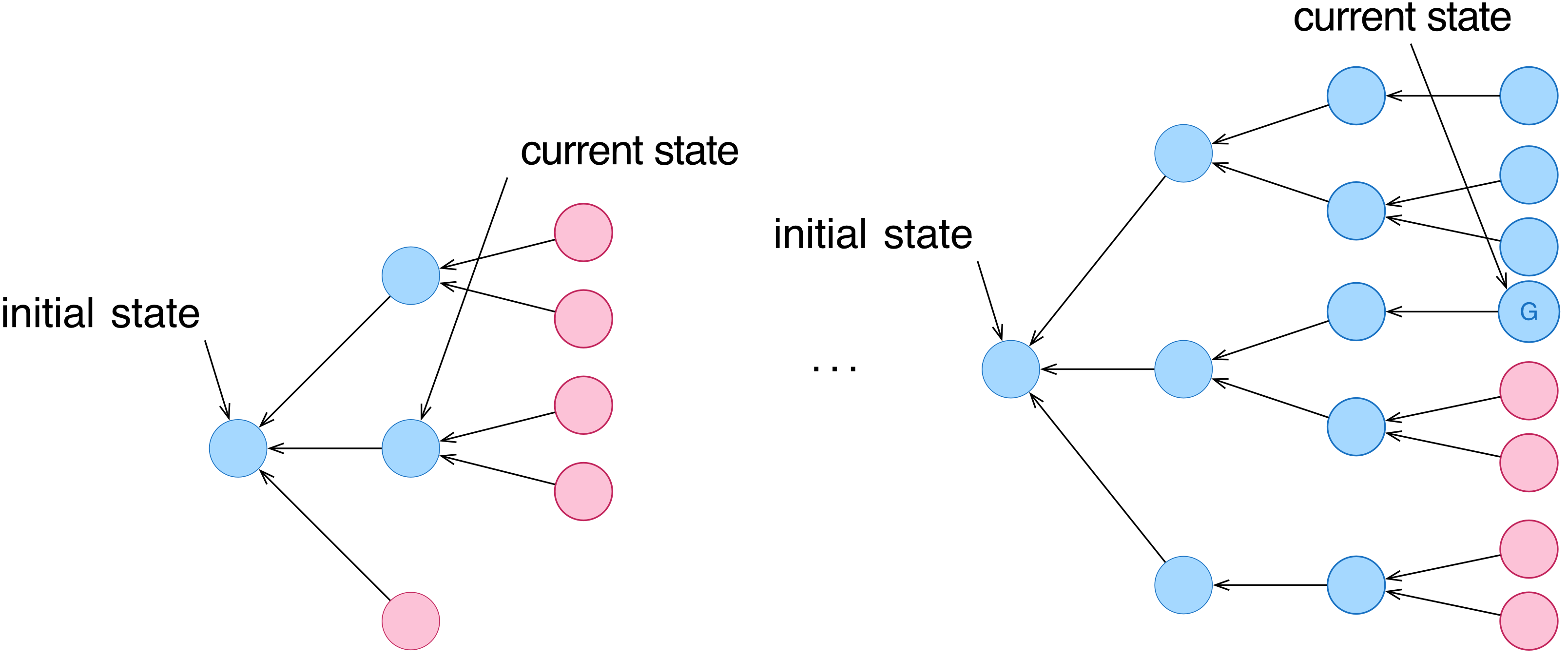
   • Repeat steps 2 and 3 until:
     • Goal test is satisfied, OR
     • Goal state is found
5. Trace Back
   
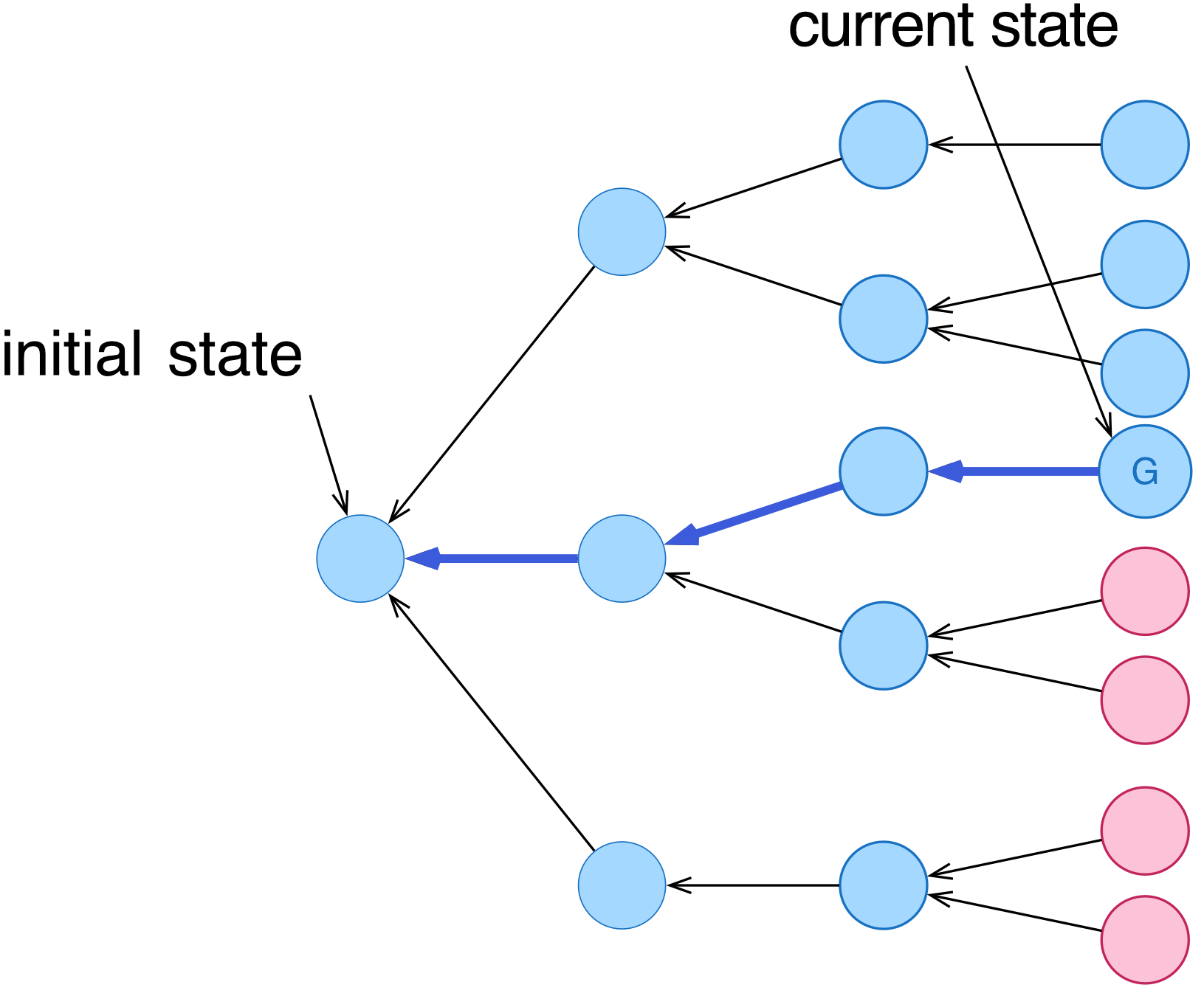
   • From goal state to initial state
   • Obtain sequence of states representing the solution

Key Insight: The order of chosen successors in the frontier affects both the solution and the performance of the search algorithm.

3.1.1 Search Tree

• Purpose: Visualize how a search is conducted
• Structure: Tree format showing state expansions

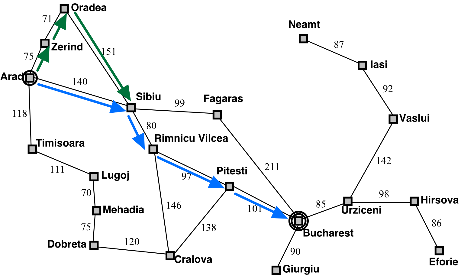
Example 3.1: Romania Route-Finding Problem

Process:

1. Start: Arad (initial state)
2. Expand Arad: → Sibiu, Timisoara, Zerind
3. Select Sibiu: → Arad, Fagaras, Oradea, Rimnicu Vilcea
4. Continue expansion until goal is reached

Solution Found: Arad → Sibiu → Rimnicu Vilcea → Pitesti → Bucharest

• การจะได้ Solution ก็คือพอถึง Goal แล้วก็ต้อง Trace Back ด้วยนะ

3.1.2 Implementing a Search Algorithm

Key Implementation Considerations

• Parent-child relationships: Must track relationships between states for solution path
• Multiple paths: A state can be reached via multiple paths
  • ลองมอง Sibiu นะ จาก Arad มันก็มีสองทางที่เขาวาดมาถูกมะ สีเขียว กับ สีน้ำเงิน
  • เราต้อง keep it separately in the memory
• Memory management: Multiple copies of states must be maintained

Node Data Structure

Each node contains:

• state: The state to which the node corresponds
• parent: The node that generates this node (a reference to parent node)
• path cost: Cumulative cost from initial node to this node
• depth: Number of steps from initial node to this node

Search Strategies

Different data structures for the frontier create different search orders:

1. Breadth-First Search (BFS)

• Data Structure: FIFO queue
• Expansion Order: Level by level
• Advantages:
  • Guarantees solution if one exists
  • Finds path with minimum number of steps
• Disadvantages:
  • Requires lots of memory
  • Must store all nodes at each level

ถ้านึกภาพเป็น Queue ก็คือ ถ้า Node ใหม่เข้ามา ก็จะถูกเป็น Node ที่ถูก explore ก่อน

2. Depth-First Search (DFS)

• Data Structure: LIFO queue (stack)
• Expansion Order: One path at a time
• Advantages:
  • Memory efficient
  • Can discard nodes in explored paths
• Disadvantages:
  • No guarantee of finding solution (if we allow revisiting visited node, stuck forever)
  • May get stuck in infinite loops with cycles

3. Depth-Limited Search

• Variant of: DFS with depth limit d (user-defined param)
• Termination: Search stops if goal not found within d steps
• Use Case: When search space is infinite or very large
• Considerations:
  • d too small → may miss existing solutions
  • d too large → may take too long to complete

4. Uniform-Cost Search (UCS)

• Data Structure: Min heap (priority queue)
• Expansion Order: Minimum path cost first
• Guarantee: Solution with minimum path cost (if all step costs ≥ 0)
• Characteristics:
  • Generalization of BFS (uses path cost instead of steps)
  • Not memory efficient
  • Must store all nodes at each level

Example 3.2: Uniform-Cost Search (Romania)

Problem: Find path from Arad to Bucharest

Process:

• Algorithm expands nodes based on lowest cumulative path cost
• Result: Requires 52 steps to reach goal state
• Implementation: Available in uninformed_search.ipynb

3.2 Graph Search

Problem with Tree Search

• States were revisited unnecessarily (e.g., Arad → Zerind → Arad)
• Reduced performance due to redundant processing

Graph Search Improvement

• Addition: "explored" set to track visited states
• Benefit: Ensures each state is processed only once
• Terminology:
  • Tree Search: Original algorithm
  • Graph Search: Modified algorithm with explored set

Example 3.3: Uniform-Cost Graph Search

Same Problem: Arad to Bucharest Improvement: More efficient by avoiding revisited states Implementation: Available in uninformed_search.ipynb

Practice Examples

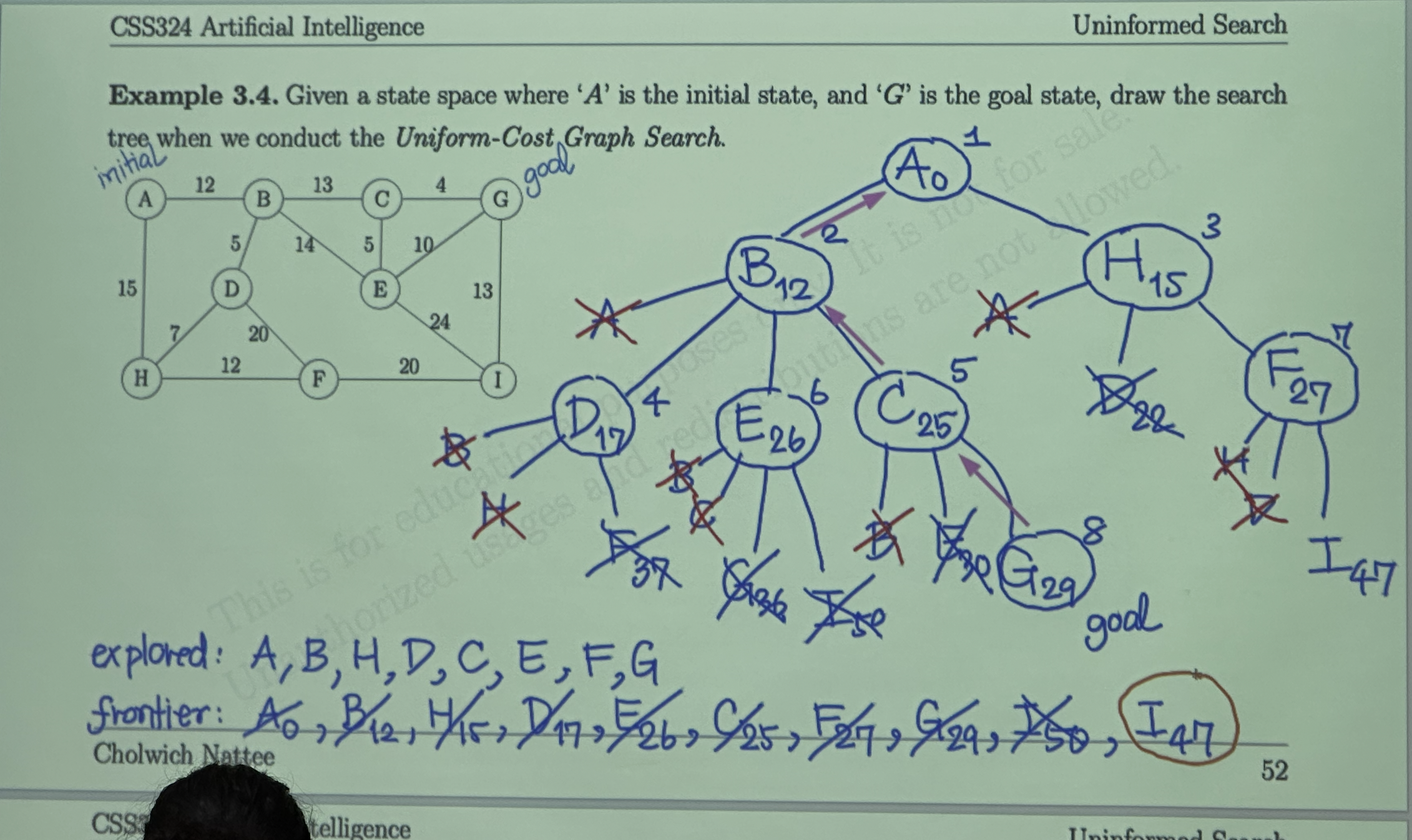
Example 3.4: State Space Search Tree

• Given: State space with initial state 'A' and goal state 'G'
• Task: Draw search tree for Uniform-Cost Graph Search
• Method: Expand nodes based on minimum cumulative cost

Example 3.5: Number Transformation Problem

• Initial State: Number 1
• Goal State: Number 10
• Available Actions:
  • Add 1 (step cost = 1)
  • Multiply by 2 (step cost = 2)
• Task: Draw search tree for Uniform-Cost Graph Search

Key Takeaways

• Search algorithms are fundamental to AI problem-solving
• Frontier management determines search strategy and performance
• Graph search is more efficient than tree search for avoiding redundant processing
• Different strategies have trade-offs between optimality, completeness, and efficiency
• Uniform-cost search guarantees optimal solutions when step costs are non-negative

ในข้อสอบมี code นะ เป็นบรรทัดโล่ง ๆ ไรงี้ ให้ fill-in-the-blanks