13 - Initial Value Problems for Ordinary Differential Equations (IVP)

ง่าย ๆ ก็คือให้ $y’(t)$ มากับ Initial condition (ค่าเริ่มต้น) แล้วหาว่า $y(t)$ ธรรมดา คือไรเอ่ย?

16 - Boundary Value Problems for Ordinary Differential Equations (BVP)

Initial Value Problems for First-Order Ordinary Differential Equations

Definition

• Consider the following problem:
  $\frac{dy}{dt} = f(t, y); \quad y(0) = y_0$
  • เรามีสมการเชิงอนุพันธ์ 1 สมการ (ฝั่งซ้ายคือ $\frac{dy}{dt}$)
  • และมี เงื่อนไขเริ่มต้น (initial condition) คือ $y(0)=y_0$
    → บอกว่า “ตอนเริ่มเวลา 0, ค่าของ y คืออะไร”
• We want to find the unknown function $y(t)$ that satisfies the above equation
  • เป้าหมาย: หาว่า $y(t)$ (ฟังก์ชันของเวลา $t$) มีหน้าตาเป็นยังไง

Examples

1. $\frac{dy}{dt} = 3t^2 y; \quad y(0) = 1$
2. $\frac{dy}{dt} = \frac{y-1}{t+3}; \quad y(0) = -1$

• These are known as initial value problems (IVP) for first-order ordinary differential equations (ODE)

Think of an IVP like knowing your starting position and speed - you're trying to figure out your entire path from there.

Types of Differential Equations

Differential Equations

• Equations with derivatives of some unknown functions

สมการที่มี อนุพันธ์ (derivative) ของฟังก์ชันที่ไม่รู้จัก

Ordinary Differential Equations (ODE)

• Differential equations where all derivatives are ordinary derivatives
• Example:
  $y\frac{d^2y}{dt^2} + \cos t \frac{dy}{dt} = e^t$

Think of ODEs like tracking how something changes over time - temperature of coffee cooling, population growth, etc.

No PARTIAL DERIVATIVE

Partial Differential Equations (PDE)

• Differential equations where some derivatives are partial derivatives
• Example:
  $\frac{\partial^2 y}{\partial t^2} = 5\frac{\partial^2 y}{\partial x^2} + xyt^2$

PDEs are like tracking how something changes across space AND time - like heat spreading across a metal plate.

มี SOME PARTIAL DERIVATIVE

First-Order ODE

สมการเชิงอนุพันธ์อันดับหนึ่ง (มีอนุพันธ์แค่ชั้นเดียว)

• ODE where all derivatives are first ordinary derivatives
• Example:
  $\frac{dy}{dt} = -t^2y^4 + e^t$
• อาจารย์บอกว่า mostly can always transform to standard form

Solving IVP Numerically

• Approximate $y(t)$ by a sequence of discrete points:
  $(t_0, y_0), (t_1, y_1), (t_2, y_2), \ldots$
  where $0 = t_0 < t_1 < t_2 < \ldots$

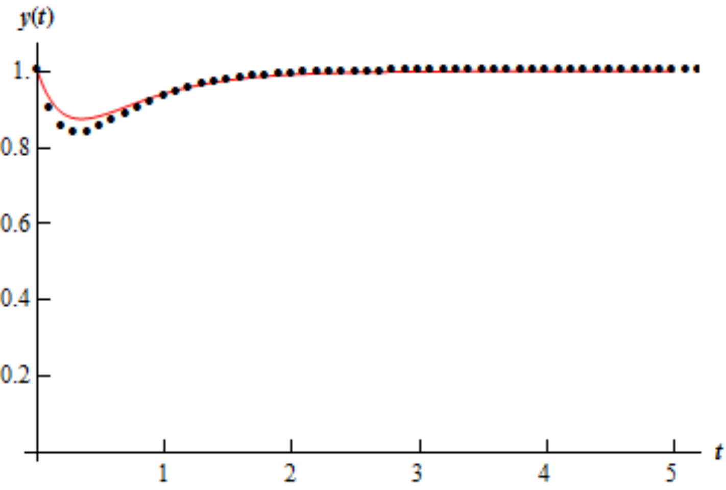
บางสมการเชิงอนุพันธ์ แก้ด้วยสูตรหรืออินทิเกรตไม่ได้จริง ๆ
ดังนั้นเราจำเป็นต้อง “ประมาณคำตอบ” ด้วย ตัวเลข (numerical method) แทน

แทนที่เราจะหาฟังก์ชัน $y(t)$ ที่ต่อเนื่องตลอดเวลา (วาดเป็นเส้นโค้งสวย ๆ)
เราจะ “แทน” มันด้วย จุด ๆ ที่คำนวณได้ทีละช่วงเวลา

"Stability" of an ODE

มันก็มี Properties ของ ODE อยู่ก็คือ Stability (แต่ไม่เหมือนกับที่เราเรียนก่อนหน้านี้นะ) ถ้าถูกต้องจริง ๆ ควรเรียกว่า Conditioning ด้วยซ้ำ

สมการนี้อ่อนไหวแค่ไหนต่อค่าตั้งต้นที่เปลี่ยนไปเล็กน้อย

Important Note

• Should be conditioning of an ODE, but traditionally (misleadingly) known as stability

Stable Solution

• A solution $y(t)$ of the ODE $y' = f(t, y)$ is stable if:
  • After perturbing the initial value (i.e., changing $y_0$ slightly)
  • The perturbed solution remains close to the original solution

Asymptotically Stable Solution

• A stable solution is asymptotically stable if:
  • Not only does the perturbed solution remain close to the original solution
  • They converge toward each other over time

Example 1.1: Stability Analysis

Problem

Is the solution to
$y' = b; \quad y(0) = y_0$
for a given real constant $b$ stable? If so, is it asymptotically stable?

Solution

• The solution to the IVP $y' = b; y(0) = y_0$ is:
  $y(t) = bt + y_0$

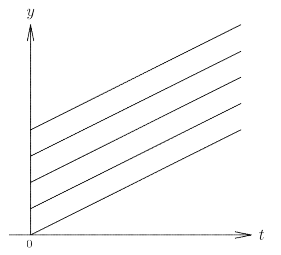
• The solution is stable but NOT asymptotically stable

Like parallel roads - they never get closer or farther apart, just stay at the same distance forever.

เจอ $y' = b$ (ค่าคงที่) → integrate ได้เลย $y = bt + C$
จากนั้นแทน initial condition หาค่า $C$
คำตอบคือ $y(t) = bt + y_0$
ซึ่ง stable แต่ไม่ asymptotically stable เพราะเส้นคู่ขนานกันตลอด

Example 1.2: Stability Analysis

รู้ว่า stable / unstable / asymptotically stable = รู้ว่า numerical method ไหนใช้ได้, step size h ควรเป็นเท่าไหร่, ใช้ explicit หรือ implicit ดี และรู้ว่าปัญหานั้น stiff ไหม

ex1.py

อาจารย์เอามาให้เรา “เห็นภาพ” ของความหมายคำว่า stable / unstable / asymptotically stable

Problem

Is the solution to
$y' = \lambda y; \quad y(0) = y_0$
for a given real constant $\lambda$ stable? If so, is it asymptotically stable?

Solution

Claim: The solution is $y = y_0 e^{\lambda t}$

Verify:
$y' = \frac{d}{dt}(y_0 e^{\lambda t}) = \lambda y_0 e^{\lambda t} = \lambda y$

and
$y(0) = y_0 e^{\lambda \cdot 0} = y_0$

Case 1: When $\lambda > 0$

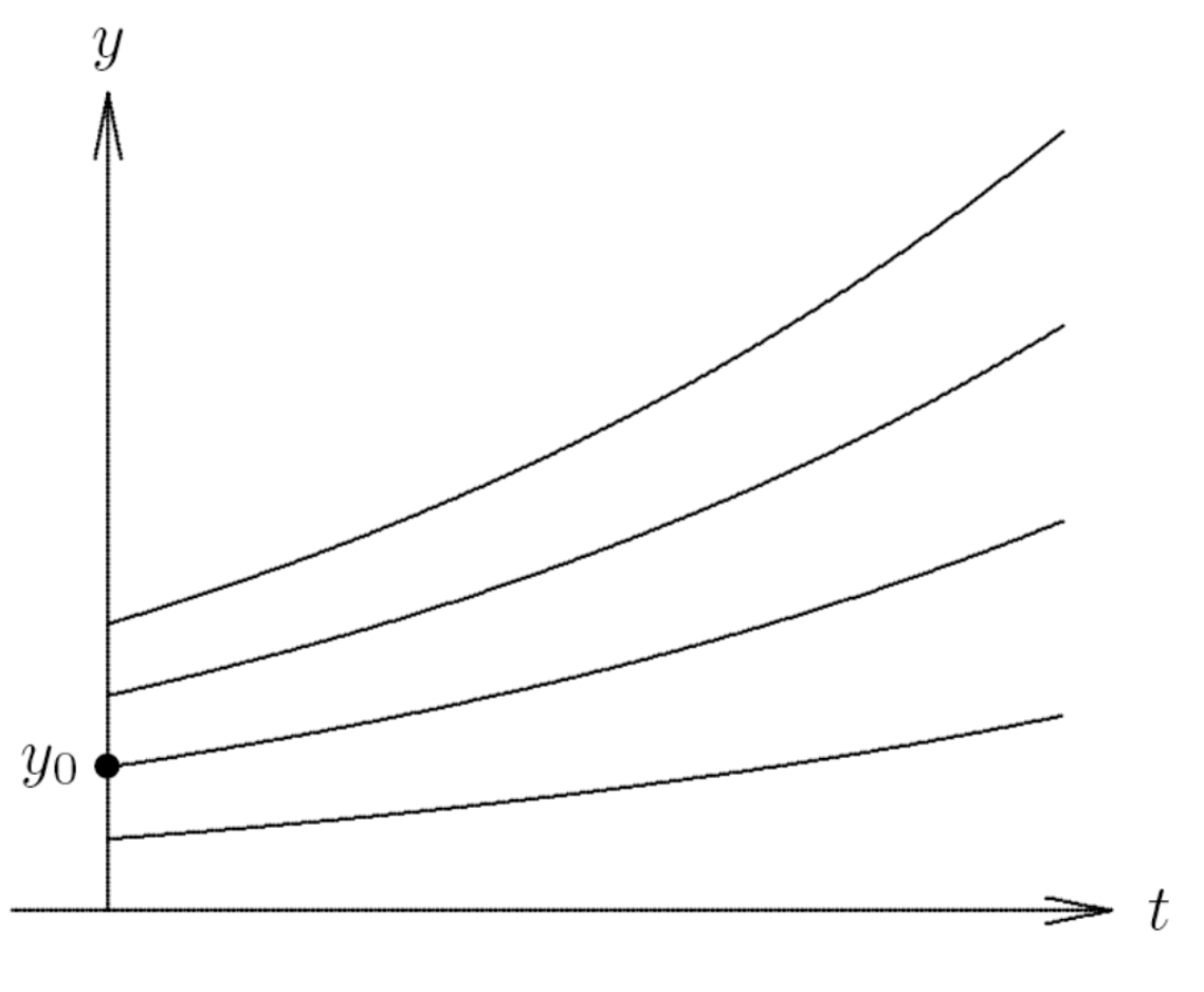
• The solution is UNSTABLE

Like compound interest - small differences in starting amounts grow exponentially over time.

Case 1: $\lambda > 0$
$e^{\lambda t}$ โตขึ้นเรื่อย ๆ เมื่อ $t$ เพิ่ม
สมมติเริ่มจาก $y_0$ ต่างกันนิดเดียว → พอเวลาผ่านไป ความต่างจะ “ขยาย” อย่างรวดเร็ว
กราฟ: เส้นโค้งชี้ขึ้นทั้งหมด → แยกออกจากกัน
สรุป: 🔴 Unstable

Case 2: When $\lambda < 0$

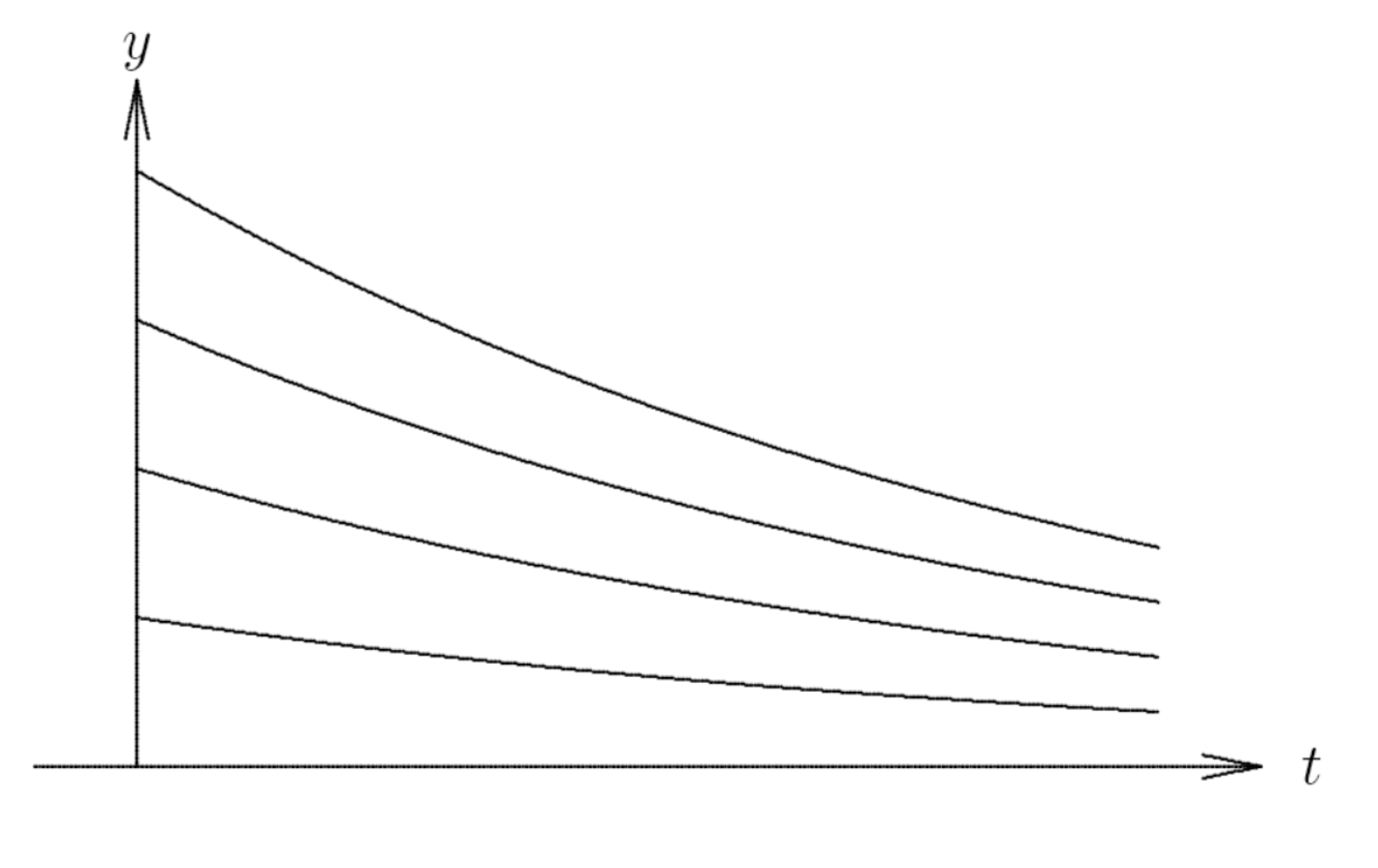
• The solution is ASYMPTOTICALLY STABLE

Like radioactive decay - all samples eventually converge toward zero, regardless of starting amount.

Case 2: $\lambda < 0$
$e^{\lambda t}$ หดลงเรื่อย ๆ (เพราะ $\lambda$ เป็นลบ → exponent ติดลบ → เข้าใกล้ 0)
ไม่ว่าค่าเริ่มต่างกันเท่าไร ทุกเส้นจะค่อย ๆ มุ่งเข้าหา $y=0$
กราฟ: เส้นโค้งที่ค่อย ๆ ลดลงจนแบนที่ศูนย์
สรุป: 🟢 Asymptotically Stable

Euler's Method

อันนี้เป็น First Method ในการ Solve First-Order ODE

Derivation

Given: $\frac{dy}{dt} = f(t, y); \quad y(0) = y_0$

Using Taylor series: